Theoretical and experimental probability offer different perspectives on the likelihood of events. At compare.edu.vn, we will explore how these probabilities are calculated and compared, offering a clear understanding of their relationship. Discover effective methods for comparing these probabilities, ensuring you grasp the nuances and applications. Uncover the secrets to statistical analysis, chance events, and predictive modeling.
1. Understanding Theoretical Probability
Theoretical probability is the expected probability of an event occurring. It is based on reasoning and calculations, not on actual experiments. The theoretical probability definition hinges on the number of favorable outcomes divided by the total number of possible outcomes, assuming all outcomes are equally likely. This form of probability is a cornerstone of probability theory and helps create probability models.
1.1 Defining Theoretical Probability
Theoretical probability is determined by analyzing the possible outcomes of an event and calculating the likelihood of a specific outcome occurring. It’s a predictive measure, indicating what should happen in an ideal scenario.
Formula:
- Theoretical Probability = (Number of Favorable Outcomes) / (Total Number of Possible Outcomes)
Example:
Consider a fair six-sided die. The theoretical probability of rolling a 3 is:
- Number of Favorable Outcomes (rolling a 3): 1
- Total Number of Possible Outcomes (rolling 1, 2, 3, 4, 5, or 6): 6
- Theoretical Probability = 1/6
This means that, theoretically, you should roll a 3 once every six rolls.
1.2 Calculating Theoretical Probability: Step-by-Step
Calculating theoretical probability involves a straightforward process:
- Identify the Sample Space: Determine all possible outcomes of the event.
- Identify Favorable Outcomes: Determine the outcomes that meet the criteria for the event you are interested in.
- Apply the Formula: Divide the number of favorable outcomes by the total number of possible outcomes.
Example: Drawing a Card from a Standard Deck
What is the theoretical probability of drawing an Ace from a standard 52-card deck?
- Sample Space: A standard deck has 52 cards.
- Favorable Outcomes: There are 4 Aces in the deck.
- Apply the Formula: Theoretical Probability = 4/52 = 1/13
Therefore, the theoretical probability of drawing an Ace is 1/13.
1.3 Examples of Theoretical Probability in Action
Understanding theoretical probability becomes clearer with practical examples:
- Coin Flip: The theoretical probability of flipping heads on a fair coin is 1/2, as there is one favorable outcome (heads) and two possible outcomes (heads or tails).
- Rolling a Die: The theoretical probability of rolling an even number on a fair six-sided die is 3/6 or 1/2, as there are three favorable outcomes (2, 4, 6) and six possible outcomes (1, 2, 3, 4, 5, 6).
- Drawing a Specific Card: The theoretical probability of drawing the Queen of Hearts from a standard deck of cards is 1/52, as there is only one Queen of Hearts in a 52-card deck.
Alt text: A clear illustration showing the formula for theoretical probability, with the numerator representing the number of favorable outcomes and the denominator representing the total number of possible outcomes.
2. Exploring Experimental Probability
Experimental probability, also known as empirical probability, is based on actual experiments and observations. It’s determined by the number of times an event occurs in an experiment relative to the total number of trials conducted. The concept of experimental probability offers a practical, real-world view of likelihood.
2.1 Defining Experimental Probability
Experimental probability is calculated by performing an experiment multiple times and recording the outcomes. It reflects what actually happened during the experiment, rather than what is expected to happen.
Formula:
- Experimental Probability = (Number of Times Event Occurs) / (Total Number of Trials)
Example:
Suppose you flip a coin 50 times and it lands on heads 28 times. The experimental probability of getting heads is:
- Number of Times Event Occurs (heads): 28
- Total Number of Trials: 50
- Experimental Probability = 28/50 = 0.56 or 56%
This means that, based on your experiment, the coin landed on heads 56% of the time.
2.2 Calculating Experimental Probability: A Practical Guide
Calculating experimental probability involves conducting an experiment and recording the results:
- Conduct the Experiment: Perform the experiment a sufficient number of times.
- Record the Outcomes: Keep track of how many times the event you’re interested in occurs.
- Apply the Formula: Divide the number of times the event occurred by the total number of trials.
Example: Rolling a Die Multiple Times
You roll a six-sided die 100 times and observe the following outcomes:
- 1: 15 times
- 2: 18 times
- 3: 16 times
- 4: 17 times
- 5: 19 times
- 6: 15 times
To find the experimental probability of rolling a 4:
- Event Occurrence: Rolling a 4 occurred 17 times.
- Total Trials: The die was rolled 100 times.
- Apply the Formula: Experimental Probability = 17/100 = 0.17 or 17%
Thus, the experimental probability of rolling a 4 is 17%.
2.3 Examples of Experimental Probability in Real-World Scenarios
Experimental probability is useful in various real-world scenarios:
- Quality Control: A manufacturer tests 500 products and finds 5 defective items. The experimental probability of a product being defective is 5/500 or 1%.
- Sports Analytics: A basketball player makes 75 out of 100 free throws. The experimental probability of the player making a free throw is 75/100 or 75%.
- Weather Forecasting: A meteorologist observes that it rains on 10 out of 30 days in April. The experimental probability of rain on any given day in April is 10/30 or 1/3.
Alt text: An example illustrating the law of large numbers, demonstrating that as the number of trials increases, the experimental probability converges toward the theoretical probability.
3. Key Differences Between Theoretical and Experimental Probability
Understanding the nuances between theoretical and experimental probability is vital for accurate statistical analysis. Theoretical probability is based on assumptions and calculations, while experimental probability is derived from real-world observations.
3.1 Source of Determination
- Theoretical Probability: Determined by logical reasoning and mathematical calculations based on the nature of the event.
- Experimental Probability: Determined by conducting experiments and observing the outcomes.
3.2 Dependence on Trials
- Theoretical Probability: Independent of the number of trials. It remains constant as it is based on the inherent properties of the event.
- Experimental Probability: Dependent on the number of trials. The more trials conducted, the closer it tends to get to the theoretical probability.
3.3 Accuracy and Ideal Conditions
- Theoretical Probability: Assumes ideal conditions (e.g., a fair coin, a balanced die). It provides an exact probability under these conditions.
- Experimental Probability: Reflects real-world conditions, which may include biases, imperfections, and random variations. It provides an approximation of the probability.
3.4 Usefulness in Different Contexts
- Theoretical Probability: Useful for predicting outcomes in controlled, idealized scenarios.
- Experimental Probability: Useful for estimating probabilities in complex, real-world scenarios where theoretical calculations are difficult or impossible.
4. How to Compare Theoretical and Experimental Probability
Comparing theoretical and experimental probabilities involves understanding their differences and using various methods to analyze and interpret them.
4.1 Identifying Scenarios for Comparison
To effectively compare theoretical and experimental probabilities, start by identifying scenarios where both can be calculated. These typically involve events with clear, defined outcomes, such as coin flips, dice rolls, or card draws.
Examples:
- Flipping a Coin: Calculate the theoretical probability of getting heads (1/2) and compare it to the experimental probability obtained after flipping the coin multiple times.
- Rolling a Die: Calculate the theoretical probability of rolling a specific number (1/6) and compare it to the experimental probability obtained after rolling the die many times.
- Drawing Cards: Calculate the theoretical probability of drawing a specific card (e.g., an Ace) and compare it to the experimental probability obtained after drawing cards from a deck with replacement.
4.2 Calculating Both Probabilities
After identifying the scenario, calculate both the theoretical and experimental probabilities:
- Theoretical Probability: Use the formula: (Number of Favorable Outcomes) / (Total Number of Possible Outcomes).
- Experimental Probability: Conduct the experiment, record the outcomes, and use the formula: (Number of Times Event Occurs) / (Total Number of Trials).
Example: Rolling a Six-Sided Die
- Theoretical Probability of Rolling a 4: 1/6
- Experimental Probability: Roll the die 100 times and record the number of times a 4 is rolled. If a 4 is rolled 18 times, the experimental probability is 18/100 or 0.18.
4.3 Comparing the Values
Once you have both probabilities, compare their values to see how closely the experimental results match the theoretical expectations. This can be done through simple subtraction, percentage difference, or graphical representation.
Methods for Comparison:
- Simple Subtraction: Subtract the experimental probability from the theoretical probability to find the difference. A smaller difference indicates a closer match.
- Percentage Difference: Calculate the percentage difference using the formula:
(|Theoretical Probability - Experimental Probability| / Theoretical Probability) * 100. - Graphical Representation: Plot the experimental probability over multiple trials and compare it to the theoretical probability line.
Example: Coin Flip Comparison
- Theoretical Probability of Heads: 0.5
- Experimental Probability After 50 Flips: 0.56
Comparison:
- Simple Subtraction: |0.5 – 0.56| = 0.06
- Percentage Difference: (|0.5 – 0.56| / 0.5) * 100 = 12%
This shows that the experimental probability differs from the theoretical probability by 0.06, or 12%.
4.4 Interpreting the Results
Interpreting the results involves understanding why the experimental probability may differ from the theoretical probability. Factors such as sample size, randomness, and biases can influence the experimental results.
Factors Influencing Differences:
- Sample Size: Smaller sample sizes are more likely to show greater deviations from the theoretical probability.
- Randomness: Random variations can occur, especially in a small number of trials.
- Biases: Biases in the experiment (e.g., a weighted die) can lead to consistent differences between theoretical and experimental probabilities.
General Guidelines for Interpretation:
- Small Differences: A small difference suggests that the experiment aligns well with theoretical expectations.
- Large Differences: A large difference may indicate that the sample size is too small, the experiment is not random, or there are biases affecting the results.
By systematically comparing theoretical and experimental probabilities, you can gain valuable insights into the nature of probability and the factors that influence experimental outcomes.
Alt text: A visual comparison highlighting the key differences between theoretical and experimental probability, emphasizing their sources and applications.
5. Factors Affecting Experimental Probability
Several factors can influence experimental probability, leading to variations from theoretical expectations. Understanding these factors is crucial for interpreting experimental results accurately.
5.1 Sample Size
The sample size, or the number of trials conducted, is a critical factor affecting experimental probability. Generally, larger sample sizes lead to experimental probabilities that are closer to the theoretical probability.
Impact of Sample Size:
- Small Sample Size: With a small number of trials, random variations can significantly impact the experimental probability. For example, flipping a coin 10 times might result in 7 heads, leading to an experimental probability of 0.7, which deviates from the theoretical probability of 0.5.
- Large Sample Size: As the number of trials increases, the effects of random variations tend to even out. Flipping a coin 1000 times is more likely to produce a result closer to 500 heads, resulting in an experimental probability closer to 0.5.
Law of Large Numbers:
The principle that as the number of trials increases, the experimental probability converges towards the theoretical probability is known as the Law of Large Numbers.
5.2 Randomness and Variability
Randomness plays a significant role in experimental probability. Even in well-controlled experiments, random variations can occur, causing the experimental probability to differ from the theoretical probability.
Sources of Random Variability:
- Inherent Randomness: Many events, such as coin flips and dice rolls, are inherently random. Each trial is independent and can produce different outcomes due to chance.
- Uncontrolled Factors: Factors that are not explicitly controlled in the experiment can introduce variability. For example, slight variations in the way a coin is flipped or a die is rolled can affect the outcome.
Managing Randomness:
- Increase Sample Size: Increasing the number of trials helps to mitigate the impact of random variability.
- Control Experiment Conditions: Minimizing uncontrolled factors can reduce variability and improve the accuracy of experimental results.
5.3 Bias in Experiments
Bias in experiments can systematically skew the results, leading to significant differences between experimental and theoretical probabilities. Bias can be introduced intentionally or unintentionally.
Types of Bias:
- Selection Bias: Occurs when the sample is not representative of the population. For example, surveying only people who frequent a particular store to estimate the popularity of a product.
- Measurement Bias: Occurs when the measurement method is flawed. For example, using a biased scale to weigh items.
- Experimenter Bias: Occurs when the experimenter influences the results, consciously or unconsciously. For example, subtly influencing participants in a study.
Mitigating Bias:
- Random Sampling: Use random sampling techniques to ensure that the sample is representative of the population.
- Calibration: Calibrate measurement tools to ensure accuracy.
- Blinding: Use blinding techniques to prevent experimenters and participants from knowing the expected outcomes.
5.4 Imperfect Instruments
Imperfect instruments or tools can introduce errors into experiments, affecting the accuracy of experimental probabilities.
Examples of Imperfect Instruments:
- Weighted Coin: A coin that is weighted on one side will not produce a 50/50 outcome when flipped.
- Unbalanced Die: A die that is not perfectly balanced will not have an equal probability of landing on each face.
- Inaccurate Measuring Devices: Rulers, scales, and other measuring devices that are not calibrated correctly can lead to measurement errors.
Addressing Imperfect Instruments:
- Calibration: Regularly calibrate instruments to ensure accuracy.
- Quality Control: Use high-quality instruments that are less prone to errors.
- Error Analysis: Account for potential errors in the analysis of experimental results.
By understanding and addressing these factors, you can improve the accuracy and reliability of experimental probabilities, making them more closely aligned with theoretical expectations.
Alt text: An illustration showing the various interrelated factors that can affect the probability of success in an experiment, highlighting the complexity of real-world scenarios.
6. Practical Applications of Probability Comparison
Comparing theoretical and experimental probabilities has numerous practical applications in various fields, providing insights into the accuracy of models and the behavior of real-world systems.
6.1 Testing Fairness of Games
One of the most straightforward applications is testing the fairness of games of chance, such as coin flips, dice rolls, and card games.
Method:
- Calculate Theoretical Probabilities: Determine the theoretical probabilities of various outcomes assuming the game is fair.
- Conduct Experiments: Perform a large number of trials and record the outcomes.
- Compare Probabilities: Compare the experimental probabilities to the theoretical probabilities.
Example: Testing a Die
- Theoretical Probabilities: For a fair six-sided die, the probability of rolling any number (1 to 6) is 1/6.
- Experiment: Roll the die 600 times and record the number of times each face appears.
- Comparison: If the experimental probabilities for each face are close to 1/6, the die is likely fair. Significant deviations may indicate that the die is weighted or biased.
Applications:
- Casinos: Ensure that games are fair and comply with regulations.
- Manufacturers: Verify the quality and balance of dice and other gaming equipment.
- Educators: Teach students about probability and statistical analysis using hands-on experiments.
6.2 Quality Control in Manufacturing
In manufacturing, comparing theoretical and experimental probabilities can help monitor and improve the quality of products.
Method:
- Establish Expected Defect Rate: Determine the theoretical defect rate based on the manufacturing process.
- Conduct Quality Checks: Sample a batch of products and inspect them for defects.
- Compare Probabilities: Compare the experimental defect rate to the expected defect rate.
Example: Electronics Manufacturing
- Expected Defect Rate: A manufacturer expects 1% of electronic components to be defective.
- Quality Check: Inspect 500 components and find 8 defective items.
- Comparison: The experimental defect rate is 8/500 = 1.6%. This is higher than the expected rate, indicating a potential issue with the manufacturing process.
Applications:
- Identify Issues: Detect problems in the manufacturing process that are causing higher-than-expected defect rates.
- Improve Processes: Implement corrective actions to reduce defects and improve product quality.
- Ensure Compliance: Meet quality standards and regulations.
6.3 Scientific Research and Experiments
In scientific research, comparing theoretical and experimental probabilities is essential for validating models and theories.
Method:
- Develop a Theoretical Model: Create a model that predicts the probabilities of various outcomes.
- Conduct Experiments: Perform experiments to collect data.
- Compare Probabilities: Compare the experimental results to the predictions of the theoretical model.
Example: Genetics
- Theoretical Model: Mendel’s laws of inheritance predict the probabilities of different traits appearing in offspring.
- Experiment: Crossbreed pea plants with different traits and observe the traits of the offspring.
- Comparison: Compare the observed ratios of traits in the offspring to the ratios predicted by Mendel’s laws.
Applications:
- Validate Theories: Confirm the validity of scientific theories and models.
- Refine Models: Identify areas where the theoretical model needs to be refined or adjusted to better match experimental results.
- Make Predictions: Use validated models to make predictions about future outcomes.
6.4 Risk Assessment in Finance and Insurance
In finance and insurance, comparing theoretical and experimental probabilities is crucial for assessing and managing risks.
Method:
- Develop Risk Models: Create models that estimate the probabilities of various risks, such as market crashes or insurance claims.
- Collect Historical Data: Gather historical data on past events.
- Compare Probabilities: Compare the predictions of the risk models to the actual outcomes observed in the historical data.
Example: Insurance
- Risk Model: An insurance company estimates the probability of a homeowner filing a claim in a given year.
- Historical Data: Collect data on the number of claims filed by homeowners over the past decade.
- Comparison: Compare the predicted number of claims to the actual number of claims.
Applications:
- Set Premiums: Determine appropriate insurance premiums based on the assessed risks.
- Manage Portfolios: Make informed investment decisions to manage financial risks.
- Comply with Regulations: Meet regulatory requirements for risk management.
By applying probability comparison in these practical scenarios, professionals can make more informed decisions, improve processes, and validate theories.
Alt text: A visualization of how probability is applied in various real-world scenarios, including weather forecasting, sports analytics, and stock market analysis.
7. Advanced Techniques for Comparing Probabilities
Beyond simple comparison, advanced statistical techniques provide deeper insights into the relationship between theoretical and experimental probabilities.
7.1 Chi-Square Test
The Chi-Square test is a statistical method used to determine if there is a significant difference between observed (experimental) and expected (theoretical) frequencies.
How it Works:
- Calculate Expected Frequencies: Determine the expected frequencies based on theoretical probabilities.
- Calculate the Chi-Square Statistic: Use the formula:
χ² = Σ [(Observed – Expected)² / Expected] - Determine Degrees of Freedom: Degrees of freedom (df) = Number of categories – 1
- Compare to Critical Value: Compare the calculated Chi-Square statistic to a critical value from a Chi-Square distribution table based on the degrees of freedom and desired significance level (e.g., 0.05).
- Interpret Results:
- If the Chi-Square statistic is greater than the critical value, reject the null hypothesis (there is a significant difference between observed and expected frequencies).
- If the Chi-Square statistic is less than the critical value, fail to reject the null hypothesis (there is no significant difference).
Example: Rolling a Die
- Theoretical Probabilities: Each face of a fair die has a probability of 1/6.
- Experiment: Roll the die 60 times and observe the following frequencies:
- 1: 8 times
- 2: 10 times
- 3: 12 times
- 4: 9 times
- 5: 11 times
- 6: 10 times
- Expected Frequencies: Each face should appear 60 * (1/6) = 10 times.
- Calculate Chi-Square Statistic:
χ² = [(8-10)²/10] + [(10-10)²/10] + [(12-10)²/10] + [(9-10)²/10] + [(11-10)²/10] + [(10-10)²/10]
χ² = 0.4 + 0 + 0.4 + 0.1 + 0.1 + 0 = 1.0 - Degrees of Freedom: df = 6 – 1 = 5
- Critical Value: For df = 5 and a significance level of 0.05, the critical value is 11.07.
- Interpretation: Since 1.0 < 11.07, we fail to reject the null hypothesis. There is no significant difference between the observed and expected frequencies.
Applications:
- Genetics: Testing if observed genetic ratios match expected Mendelian ratios.
- Marketing: Analyzing if observed customer preferences match expected preferences.
- Social Sciences: Determining if observed survey results match expected distributions.
7.2 Hypothesis Testing
Hypothesis testing is a formal procedure for making decisions about statistical hypotheses based on sample data. It involves setting up a null hypothesis (H0) and an alternative hypothesis (H1) and then determining whether the data provide enough evidence to reject the null hypothesis.
Steps in Hypothesis Testing:
- State the Hypotheses:
- Null Hypothesis (H0): A statement of no effect or no difference.
- Alternative Hypothesis (H1): A statement that contradicts the null hypothesis.
- Choose a Significance Level (α): The probability of rejecting the null hypothesis when it is true (Type I error). Common values are 0.05 and 0.01.
- Calculate a Test Statistic: A value calculated from the sample data that is used to determine whether to reject the null hypothesis.
- Determine the P-value: The probability of obtaining a test statistic as extreme as, or more extreme than, the one calculated from the sample data, assuming the null hypothesis is true.
- Make a Decision:
- If the P-value is less than or equal to the significance level (α), reject the null hypothesis.
- If the P-value is greater than the significance level (α), fail to reject the null hypothesis.
Example: Testing a Coin for Fairness
- Hypotheses:
- H0: The coin is fair (probability of heads = 0.5).
- H1: The coin is not fair (probability of heads ≠ 0.5).
- Significance Level: α = 0.05
- Experiment: Flip the coin 100 times and observe 60 heads.
- Test Statistic: Use a z-test for proportions:
z = (p – P) / √(P(1-P)/n)
where:
p = sample proportion (60/100 = 0.6)
P = hypothesized proportion (0.5)
n = sample size (100)
z = (0.6 – 0.5) / √(0.5(1-0.5)/100) = 2 - P-value: For a two-tailed test with z = 2, the P-value is approximately 0.0455.
- Decision: Since 0.0455 < 0.05, we reject the null hypothesis. There is evidence to suggest that the coin is not fair.
Applications:
- Clinical Trials: Determining if a new drug is more effective than a placebo.
- Market Research: Analyzing if a new marketing campaign has increased sales.
- Environmental Science: Assessing if pollution levels have changed over time.
7.3 Confidence Intervals
A confidence interval is a range of values that is likely to contain the true value of a population parameter with a certain level of confidence.
How to Construct a Confidence Interval:
- Choose a Confidence Level: The desired level of confidence (e.g., 95%, 99%).
- Calculate the Sample Statistic: The point estimate of the population parameter (e.g., sample mean, sample proportion).
- Determine the Margin of Error: The amount added and subtracted from the sample statistic to create the interval. The margin of error depends on the confidence level, sample size, and standard deviation.
- Construct the Interval:
Confidence Interval = Sample Statistic ± Margin of Error
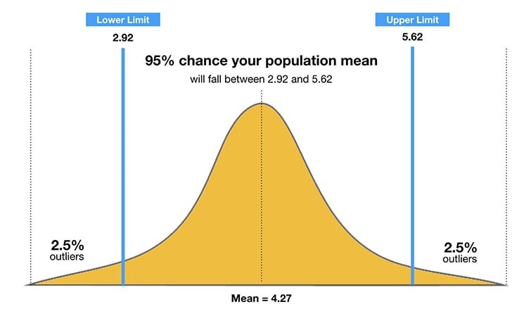
Example: Estimating the Proportion of Voters Supporting a Candidate
- Confidence Level: 95%
- Sample: Survey 400 voters and find that 220 support the candidate.
- Sample Proportion: p = 220/400 = 0.55
- Margin of Error: For a 95% confidence level, the critical value (z) is approximately 1.96. The margin of error is:
Margin of Error = z √(p(1-p)/n) = 1.96 √(0.55(1-0.55)/400) ≈ 0.048 - Confidence Interval:
Confidence Interval = 0.55 ± 0.048 = (0.502, 0.598)
Interpretation:
We are 95% confident that the true proportion of voters supporting the candidate is between 50.2% and 59.8%.
Applications:
- Political Polling: Estimating the proportion of voters supporting a candidate.
- Market Research: Determining the proportion of consumers who prefer a particular product.
- Healthcare: Estimating the effectiveness of a medical treatment.
By using these advanced techniques, researchers and analysts can gain a deeper understanding of the relationship between theoretical and experimental probabilities, leading to more accurate conclusions and informed decisions.
 Advanced techniques for comparing probabilities
Alt text: A visual representation of a confidence interval, illustrating how it provides a range within which the true population parameter is likely to fall.
8. Tools and Resources for Probability Comparison
Several tools and resources can aid in comparing theoretical and experimental probabilities, enhancing the accuracy and efficiency of the analysis.
8.1 Statistical Software Packages
Statistical software packages provide a wide range of functions for calculating probabilities, performing statistical tests, and creating visualizations.
Examples:
- R: A free, open-source programming language and software environment for statistical computing and graphics. R is highly extensible and supports a wide range of statistical techniques.
- Features: Hypothesis testing, regression analysis, data visualization, and more.
- Use Case: Analyzing experimental data and comparing it to theoretical models.
- Python (with Libraries): Python, with libraries like NumPy, SciPy, and Matplotlib, provides powerful tools for statistical analysis and data visualization.
- Features: Statistical functions, data manipulation, plotting, and more.
- Use Case: Conducting simulations, performing statistical tests, and visualizing experimental results.
- SPSS: A widely used statistical software package for data analysis and management.
- Features: Descriptive statistics, hypothesis testing, regression analysis, and more.
- Use Case: Analyzing survey data and comparing observed distributions to expected distributions.
- SAS: A comprehensive statistical software suite for advanced analytics, business intelligence, and data management.
- Features: Statistical modeling, data mining, forecasting, and more.
- Use Case: Analyzing complex datasets and building predictive models.
8.2 Online Calculators
Online calculators offer convenient tools for performing basic probability calculations and statistical tests.
Examples:
- Chi-Square Calculator: Calculates the Chi-Square statistic and P-value for categorical data.
- Use Case: Determining if there is a significant difference between observed and expected frequencies.
- Hypothesis Testing Calculator: Performs hypothesis tests for means, proportions, and variances.
- Use Case: Testing if a sample mean is significantly different from a hypothesized population mean.
- Confidence Interval Calculator: Calculates confidence intervals for means, proportions, and variances.
- Use Case: Estimating the range of values that is likely to contain the true population parameter.
Benefits:
- Accessibility: Available online from any device with an internet connection.
- Ease of Use: Simple and intuitive interfaces make them easy to use, even for those with limited statistical knowledge.
- Speed: Provide quick and accurate results.
8.3 Educational Websites and Courses
Educational websites and courses offer resources for learning about probability, statistics, and data analysis.
Examples:
- Khan Academy: Provides free video lessons and practice exercises on a wide range of topics, including probability and statistics.
- Features: Interactive lessons, practice problems, and progress tracking.
- Use Case: Learning the fundamentals of probability and statistics.
- Coursera: Offers online courses and specializations from top universities and institutions.
- Features: Video lectures, assignments, and certificates of completion.
- Use Case: Taking in-depth courses on statistical analysis and data science.
- edX: Provides online courses and programs from leading universities and institutions.
- Features: Video lectures, quizzes, and certificates of completion.
- Use Case: Learning advanced statistical techniques and data analysis methods.
- Statistics.com: Offers online courses and workshops on a variety of statistical topics.
- Features: Expert instructors, hands-on exercises, and personalized feedback.
- Use Case: Developing practical skills in statistical analysis.
8.4 Simulation Tools
Simulation tools allow you to create and run simulations to model random events and observe the outcomes.
Examples:
- Monte Carlo Simulation Software: Uses random sampling to model the probability of different outcomes in a process that cannot easily be predicted due to the intervention of random variables.
- Use Case: Simulating the outcomes of complex systems, such as financial markets or weather patterns.
- Online Simulation Tools: Several websites offer online tools for simulating coin flips, dice rolls, and other random events.
- Use Case: Visualizing the effects of sample size and randomness on experimental probabilities.
By leveraging these tools and resources, you can effectively compare theoretical and experimental probabilities, gain deeper insights into the nature of randomness, and make more informed decisions based on data.
Alt text: A visual representation of a Monte Carlo simulation, showing how random sampling is used to estimate the probability of different outcomes.
9. Common Mistakes to Avoid When Comparing Probabilities
Comparing theoretical and experimental probabilities can be tricky, and avoiding common mistakes is crucial for accurate analysis and interpretation.
9.1 Insufficient Sample Size
One of the most common mistakes is using an insufficient sample size. Small sample sizes can lead to experimental probabilities that deviate significantly from theoretical probabilities due to random variations.
Example:
Flipping a coin only 10 times may result in 7 heads, leading to an experimental probability of 0.7, which is quite different from the theoretical probability of 0.5.
How to Avoid:
- Increase the Sample Size: Ensure that you conduct enough trials to minimize the impact of random variations. The Law of Large Numbers states that as the number of trials increases, the experimental probability will converge towards the theoretical probability.
- Use Statistical Power Analysis: Perform a power analysis to determine the minimum sample size needed to detect a statistically significant difference between the experimental and theoretical probabilities.
9.2 Ignoring Potential Biases
Failing to account for potential biases in the experiment can lead to skewed results and inaccurate comparisons.
Example:
Using a weighted coin will result in experimental probabilities that consistently favor one side over the other, deviating from the theoretical expectation of a fair coin.
How to Avoid:
- Random Sampling: Use random sampling techniques to ensure that the sample is representative of the population.
- Calibration: Calibrate measurement tools to ensure accuracy.
- Blinding: Use blinding techniques to prevent experimenters and participants from knowing the expected outcomes.
- Control for Confounding Variables: Identify and control for variables that could influence the results.
9.3 Misinterpreting Statistical Significance
Confusing statistical significance with practical significance can lead to incorrect conclusions. A statistically significant result may not always be practically meaningful.
Example:
A clinical trial finds that a new drug is statistically significantly more effective than a placebo, but the improvement in symptoms is minimal and may not justify the drug’s cost and side effects.
How to Avoid:
- Consider Effect Size: Evaluate the magnitude of the effect, not just the statistical significance.
- Use Confidence Intervals: Provide