How to Compare Similar Data in Excel: A Guide

Comparing similar data in Excel can be a daunting task, but COMPARE.EDU.VN offers solutions to streamline the process and ensure accuracy. This guide provides comprehensive methods on How To Compare Similar Data In Excel effectively, focusing on different techniques and scenarios, ultimately providing insights into data comparison and analysis in Excel. Leverage data comparison tools to make informed decisions with ease.

1. Understanding the Need to Compare Similar Data in Excel

Data comparison is crucial in various fields, from finance and accounting to marketing and sales. In Excel, the ability to compare similar datasets enables users to identify discrepancies, track changes, and ensure data integrity. Whether you’re comparing product lists, financial statements, or customer databases, knowing how to effectively compare similar data in Excel is an invaluable skill.

1.1. Why is Data Comparison Important?

Effective data comparison helps in:

Identifying Errors: Spotting inconsistencies and mistakes in datasets.
Tracking Changes: Monitoring how data evolves over time.
Ensuring Accuracy: Verifying the reliability of data.
Making Informed Decisions: Providing a solid foundation for strategic choices.
Maintaining Data Integrity: Keeping data consistent and trustworthy across different sources.

1.2. Scenarios Where Data Comparison is Essential

Financial Analysis: Comparing budget vs. actual figures to identify variances.
Sales and Marketing: Tracking campaign performance across different periods.
Inventory Management: Ensuring accurate stock levels by comparing records.
Customer Relationship Management (CRM): Identifying duplicate entries and updating customer information.
Academic Research: Comparing experimental data to validate findings.

2. Preparing Your Data for Comparison

Before diving into the techniques, ensure your data is well-prepared for comparison. This involves cleaning, organizing, and formatting your data to facilitate accurate and efficient analysis.

2.1. Data Cleaning Techniques

Removing Duplicates: Use Excel’s “Remove Duplicates” feature to eliminate redundant entries.
Standardizing Formats: Ensure consistent date, number, and text formats.
Handling Missing Values: Decide how to treat blank cells (e.g., replace with zero, leave blank, or fill with a placeholder).
Correcting Errors: Manually fix any obvious typos or inconsistencies.
Trimming Spaces: Remove leading and trailing spaces using the TRIM function.

2.2. Organizing Data for Comparison

Consistent Column Headers: Ensure column headers are clear, consistent, and descriptive.
Sorting Data: Sort data based on relevant criteria (e.g., date, product ID) to facilitate comparison.
Using Tables: Convert your data ranges into Excel tables for easier management and dynamic formula referencing.

2.3. Formatting Data for Readability

Conditional Formatting: Use color scales, data bars, and icon sets to highlight differences and patterns.
Number Formatting: Apply appropriate number formats (e.g., currency, percentage) for clarity.
Cell Styles: Use cell styles to visually group and categorize data.
Font and Alignment: Choose readable fonts and proper alignment for ease of reading.

3. Basic Techniques to Compare Similar Data in Excel

Excel offers several built-in features and formulas to compare similar data effectively. These range from simple visual comparisons to more advanced formula-based techniques.

3.1. Visual Comparison

Visual comparison involves manually scanning datasets for differences. While this method is straightforward, it’s best suited for small datasets or initial assessments.

Sorting and Filtering: Sort and filter data to group similar items together, making it easier to spot differences.
Side-by-Side Comparison: Arrange the datasets side-by-side on the screen for direct visual inspection.
Using Different Colors: Manually highlight cells or rows with different values to draw attention to discrepancies.

3.2. Conditional Formatting

Conditional formatting is a powerful tool for highlighting differences and patterns in your data based on specific criteria.

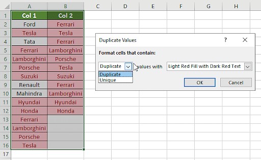
3.2.1. Highlighting Duplicate Values

How to Use: Select the data range, go to “Home” > “Conditional Formatting” > “Highlight Cells Rules” > “Duplicate Values.”
Use Case: Identifying duplicate entries in a customer list or product catalog.

3.2.2. Highlighting Unique Values

How to Use: Select the data range, go to “Home” > “Conditional Formatting” > “Highlight Cells Rules” > “Unique Values.”
Use Case: Identifying unique product IDs or customer accounts.

3.2.3. Using Formula-Based Conditional Formatting

How to Use: Select the data range, go to “Home” > “Conditional Formatting” > “New Rule” > “Use a formula to determine which cells to format.”
Use Case: Highlighting rows where values in two columns do not match.

3.3. Using the Equals Operator (=)

The equals operator is a simple way to compare corresponding cells in two columns and return TRUE if they match or FALSE if they don’t.

How to Use: In a new column, enter a formula like =A1=B1.
Use Case: Quick comparison of two columns to identify matching entries.

3.4. Using the IF Formula

The IF formula allows you to perform a logical test and return different values based on whether the test is TRUE or FALSE.

How to Use: =IF(A1=B1, "Match", "Mismatch")
Use Case: Providing custom messages for matching and non-matching entries.

3.5. Using the EXACT Formula

The EXACT formula compares two text strings and returns TRUE only if they are identical, including case.

How to Use: =EXACT(A1, B1)
Use Case: Case-sensitive comparison of text data.

4. Advanced Techniques for Data Comparison

For more complex data comparison tasks, Excel offers advanced formulas and functions that provide greater flexibility and precision.

4.1. Using the VLOOKUP Function

The VLOOKUP function searches for a value in the first column of a table and returns a value in the same row from another column.

How to Use: =VLOOKUP(lookup_value, table_array, col_index_num, [range_lookup])
Use Case: Comparing two lists and finding matching data or identifying values present in one list but not the other.

4.2. Using the INDEX and MATCH Functions

The INDEX and MATCH functions can be combined to perform more flexible lookups than VLOOKUP. MATCH finds the position of a value in a range, and INDEX returns the value at that position in another range.

How to Use: =INDEX(return_range, MATCH(lookup_value, lookup_range, 0))
Use Case: Similar to VLOOKUP, but more flexible because you can look up values based on criteria in any column, not just the first.

4.3. Using the COUNTIF Function

The COUNTIF function counts the number of cells within a range that meet a given criterion.

How to Use: =COUNTIF(range, criteria)
Use Case: Determining how many times a value from one column appears in another column.

4.4. Using the SUMIF Function

The SUMIF function sums the values in a range that meet a given criterion.

How to Use: =SUMIF(range, criteria, sum_range)
Use Case: Summing values in one column based on matching values in another column.

4.5. Using Array Formulas

Array formulas can perform complex calculations on multiple values at once. They are entered by pressing Ctrl + Shift + Enter.

How to Use: Enter the formula and press Ctrl + Shift + Enter.
Use Case: Comparing entire ranges of data and performing calculations based on the comparison results.

5. Comparing Multiple Columns Simultaneously

When you need to compare more than two columns, Excel offers several techniques to streamline the process and provide comprehensive insights.

5.1. Using the AND Function

The AND function checks whether all conditions in a test are TRUE.

How to Use: =AND(A1=B1, A1=C1, B1=C1)
Use Case: Verifying that values in multiple columns are identical.

5.2. Using the OR Function

The OR function checks whether at least one condition in a test is TRUE.

How to Use: =OR(A1=B1, A1=C1, B1=C1)
Use Case: Identifying rows where at least two columns have matching values.

5.3. Using the COUNTIFS Function

The COUNTIFS function counts the number of cells that meet multiple criteria.

How to Use: =COUNTIFS(range1, criteria1, range2, criteria2, ...)
Use Case: Counting rows where multiple columns meet specific criteria.

5.4. Creating Helper Columns

Helper columns involve adding additional columns to your data to perform intermediate calculations or comparisons, making it easier to analyze the results.

How to Use: Create new columns with formulas that perform specific comparisons, then analyze the results in these columns.
Use Case: Breaking down complex comparisons into smaller, more manageable steps.

6. Real-World Examples and Use Cases

To illustrate the practical applications of these techniques, let’s explore some real-world examples where comparing similar data in Excel is essential.

6.1. Financial Analysis: Budget vs. Actual

Scenario: Comparing budgeted expenses against actual expenses to identify variances.
Techniques Used: IF formula, conditional formatting, SUMIF function.
Steps:
1. Create columns for budgeted expenses and actual expenses.
2. Use the IF formula to calculate the variance (e.g., =IF(B2>A2, "Over Budget", "Under Budget")).
3. Use conditional formatting to highlight variances above a certain threshold.
4. Use the SUMIF function to summarize total variances by category.

6.2. Sales and Marketing: Campaign Performance

Scenario: Tracking the performance of marketing campaigns across different channels.
Techniques Used: VLOOKUP function, pivot tables, conditional formatting.
Steps:
1. Create a table with campaign data, including metrics like impressions, clicks, and conversions.
2. Use the VLOOKUP function to pull in cost data from a separate budget table.
3. Create a pivot table to summarize campaign performance by channel.
4. Use conditional formatting to highlight top-performing and underperforming campaigns.

6.3. Inventory Management: Stock Levels

Scenario: Comparing current stock levels against reorder points to identify items that need to be reordered.
Techniques Used: IF formula, conditional formatting.
Steps:
1. Create columns for current stock levels and reorder points.
2. Use the IF formula to identify items below the reorder point (e.g., =IF(A2<B2, "Reorder", "")).
3. Use conditional formatting to highlight items that need to be reordered.

6.4. Customer Relationship Management (CRM): Duplicate Entries

Scenario: Identifying and merging duplicate customer records.
Techniques Used: Conditional formatting, COUNTIF function.
Steps:
1. Use conditional formatting to highlight duplicate email addresses or phone numbers.
2. Use the COUNTIF function to count the number of times each email address or phone number appears in the list.
3. Manually review the highlighted records and merge duplicates.

7. Best Practices for Data Comparison in Excel

To ensure accurate and efficient data comparison, follow these best practices:

Plan Your Comparison: Define your objectives and identify the key metrics you want to compare.
Prepare Your Data: Clean, organize, and format your data before starting the comparison.
Choose the Right Technique: Select the most appropriate method based on the size and complexity of your data.
Validate Your Results: Double-check your formulas and results to ensure accuracy.
Document Your Process: Keep a record of the steps you took to compare the data, including any formulas or conditional formatting rules you used.
Use Clear and Descriptive Labels: Ensure that your columns and rows have clear, descriptive labels to make the data easy to understand.
Automate Repetitive Tasks: Use macros or Power Query to automate repetitive data comparison tasks.

8. Troubleshooting Common Issues

Even with careful planning and execution, you may encounter issues when comparing similar data in Excel. Here are some common problems and how to troubleshoot them:

Formulas Not Working:
- Check for syntax errors in your formulas.
- Ensure that cell references are correct.
- Make sure array formulas are entered correctly (using Ctrl + Shift + Enter).
Incorrect Results:
- Double-check your data for inconsistencies or errors.
- Verify that your conditional formatting rules are set up correctly.
- Review your formulas to ensure they are performing the intended calculations.
Performance Issues:
- Avoid using complex formulas on large datasets.
- Use Excel tables to improve performance.
- Close unnecessary applications to free up system resources.
Unexpected Errors:
- Save your workbook frequently to avoid data loss.
- Restart Excel or your computer if you encounter persistent errors.
- Check for updates to Excel to ensure you have the latest bug fixes and performance improvements.

9. Leveraging COMPARE.EDU.VN for Data Comparison

While Excel is a powerful tool for data comparison, COMPARE.EDU.VN offers additional resources and services to enhance your capabilities.

9.1. Access to Expert Reviews and Comparisons

COMPARE.EDU.VN provides expert reviews and comparisons of various products, services, and software, including data analysis tools and Excel add-ins. These reviews can help you identify the best solutions for your specific data comparison needs.

9.2. Step-by-Step Tutorials and Guides

COMPARE.EDU.VN offers step-by-step tutorials and guides on various data analysis topics, including data comparison in Excel. These resources can help you learn new techniques and improve your skills.

9.3. Community Forum for Sharing Tips and Best Practices

COMPARE.EDU.VN hosts a community forum where you can connect with other data analysts and Excel users to share tips, best practices, and solutions to common problems. This forum is a valuable resource for learning from others and staying up-to-date on the latest trends and techniques.

10. Frequently Asked Questions (FAQs)

10.1. How do I compare two columns in Excel and highlight the differences?

Use conditional formatting with a formula. Select your data, go to “Conditional Formatting” > “New Rule” > “Use a formula to determine which cells to format.” Enter a formula like =A1<>B1 and choose a format to highlight the differences.

10.2. Can I compare two columns in Excel for partial matches?

Yes, you can use the SEARCH or FIND functions to check for partial matches. For example, =IF(ISNUMBER(SEARCH(B1, A1)), "Partial Match", "No Match") checks if the value in B1 is found within the value in A1.

10.3. How can I compare data from two different Excel files?

You can use VLOOKUP or INDEX/MATCH to compare data between two Excel files. Make sure both files are open, and reference the data in the other file by including the file name in the formula.

10.4. Is there a way to automate data comparison in Excel?

Yes, you can use macros or Power Query to automate data comparison tasks. Macros allow you to record and replay a series of actions, while Power Query allows you to import and transform data from multiple sources.

10.5. How do I handle errors when comparing data in Excel?

Use the IFERROR function to handle errors. For example, =IFERROR(VLOOKUP(A1, B:C, 2, FALSE), "Not Found") returns “Not Found” if the VLOOKUP function returns an error.

10.6. What is the best way to compare large datasets in Excel?

For large datasets, consider using Power Query or Power Pivot. These tools can handle large amounts of data more efficiently than standard Excel formulas.

10.7. How do I compare two lists and pull matching data?

Use the VLOOKUP function or the INDEX/MATCH combination. =VLOOKUP(D2, $A$2:$B$6, 2, FALSE) will find the matching data.

10.8. Can I compare two columns for case-sensitive matches?

Yes, use the EXACT formula. =EXACT(A2, B2) will return TRUE only if the values are exactly the same, including case.

10.9. How do I compare multiple columns for row matches?

Use the AND function. =IF(AND(A2=B2, A2=C2), "Complete match", " ") will check if all columns match.

10.10. How can I highlight row matches and differences?

You can create a conditional formatting formula that can highlight the rows that include identical values in all the columns. You can use the following formula for the desired result: =AND($A2=$B2, $A2=$C2) or =COUNTIF($A2:$C2, $A2)=3

Conclusion

Comparing similar data in Excel is a critical skill for data analysis, decision-making, and maintaining data integrity. By mastering the techniques and best practices outlined in this guide, you can streamline your data comparison tasks, identify errors, track changes, and ensure the accuracy of your data.

Remember to leverage the resources available at COMPARE.EDU.VN, including expert reviews, tutorials, and community forums, to enhance your data analysis capabilities.

Ready to take your data comparison skills to the next level? Visit COMPARE.EDU.VN today to explore more tutorials, reviews, and resources. Make informed decisions and ensure data accuracy with our comprehensive guides. Contact us at 333 Comparison Plaza, Choice City, CA 90210, United States, or reach out via WhatsApp at +1 (626) 555-9090. Let compare.edu.vn be your trusted partner in data analysis.