How to Compare Rows in Two Different Excel Sheets

Comparing data across two Excel sheets can be tedious, especially with large datasets. This article provides a step-by-step guide on how to efficiently compare rows in two different Excel sheets to identify discrepancies and highlight changes. We’ll leverage helper columns, concatenation, and conditional formatting to streamline this process.

Using a Helper Column to Concatenate Data

The key to comparing entire rows efficiently is to consolidate all relevant data within each row into a single string. We achieve this by using a “helper column” and the concatenation function.

1. Choose a Helper Column: Select an empty column outside your data range. For instance, if your data spans columns A to AX, you could use column AZ as your helper column.

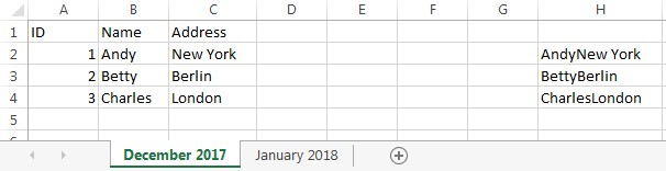
2. Concatenate Row Data: In the first cell of your helper column (e.g., AZ2), enter a formula that concatenates the data from all relevant cells in that row. Use the ampersand symbol (&) to join the cell values:

   =B2&C2&D2&…&AX2

   This formula combines the values from B2 to AX2 into a single string. If your data might contain values that could lead to false negatives when comparing (e.g., “the” and “react” changing to “there” and “act”), consider adding a delimiter like a pipe symbol (|) between each cell value:

   =B2&"|"&C2&"|"&D2&"|"&…&"|"&AX2

3. Apply the Formula to All Rows: Drag the fill handle (the small square at the bottom right of the cell) down to apply the formula to all rows in your data. Repeat this process for both Excel sheets.

Applying Conditional Formatting to Highlight Differences

Now that we have consolidated row data, we can use conditional formatting to pinpoint discrepancies between the two sheets.

1. Select the Target Range: On the sheet where you want to highlight changes (typically the newer sheet), select the cells you want to format. This could be a single column (e.g., Column A for ID) or the entire data range.

2. Create a New Conditional Formatting Rule: Go to “Conditional Formatting” -> “New Rule…”.

3. Use a Formula: Choose “Use a formula to determine which cells to format”.

4. Enter the Comparison Formula: In the formula input box, enter a formula that compares the concatenated data in the current sheet with the corresponding data in the previous sheet using VLOOKUP. This formula assumes your ID is in column A:

    =IFERROR(VLOOKUP($A2,'[Previous Sheet Name]'!$A$2:$AZ$1200,52,FALSE), "") <> $AZ2

   Replace [Previous Sheet Name] with the actual name of your previous sheet, 52 with the column number of your helper column (AZ in this example), and 1200 with a row number that encompasses all your data in the previous sheet.

5. Set the Formatting: Click on “Format…” and choose the desired formatting for highlighting differences (e.g., orange fill).

Conclusion

By utilizing helper columns, concatenation, and conditional formatting, you can effectively compare rows across two Excel sheets and quickly identify any discrepancies. This method simplifies data analysis and allows for efficient tracking of changes between datasets. Remember to adapt the formulas to your specific spreadsheet structure and data range for accurate results. Once you have the conditional formatting set up, you can hide the helper columns to maintain a cleaner view of your data.