Comparing a single value against multiple values in Excel is a common task that can be accomplished in several ways, allowing you to identify matches, determine if a value falls within a range, or perform other types of comparative analysis. At COMPARE.EDU.VN, we understand the need for clear and effective methods to achieve this. This article will explore various techniques for comparing one value with multiple values in Excel, ensuring you have the tools to make informed decisions. Let’s delve into the strategies that can help you compare data effectively and efficiently using Excel.
1. Understanding the Need for Comparison in Excel
In Excel, comparing a single value with multiple values is essential for a variety of reasons. Whether you are analyzing sales data, managing inventory, or tracking financial performance, the ability to compare data accurately and efficiently is critical for making informed decisions.
- Data Validation: Ensuring data entries meet specific criteria.
- Performance Tracking: Comparing current performance against targets.
- Anomaly Detection: Identifying unusual values that deviate from the norm.
- Decision Making: Evaluating options based on comparative data.
2. Basic Comparison Techniques
Before diving into more advanced methods, let’s cover some basic techniques for comparing values in Excel.
2.1. Using the IF Function
The IF function is a fundamental tool for performing comparisons in Excel. It allows you to test a condition and return one value if the condition is true and another value if the condition is false.
=IF(A1>B1,"A1 is greater","B1 is greater or equal")This formula compares the value in cell A1 with the value in cell B1. If A1 is greater than B1, it returns “A1 is greater”; otherwise, it returns “B1 is greater or equal.”
2.2. Using Comparison Operators
Excel provides several comparison operators that can be used within formulas:
=: Equal to>: Greater than<: Less than>=: Greater than or equal to<=: Less than or equal to<>: Not equal to
These operators can be combined with the IF function or other functions to create more complex comparisons.
3. Comparing One Value with a Range of Values
One common scenario is comparing a single value against a range of values to determine if it falls within that range or meets specific criteria.
3.1. Using the AND and OR Functions
The AND and OR functions can be used to create more complex conditions for comparison.
AND(condition1, condition2, ...): ReturnsTRUEif all conditions are true.OR(condition1, condition2, ...): ReturnsTRUEif at least one condition is true.
For example, to check if a value in cell A1 is between 10 and 20, you can use the following formula:
=IF(AND(A1>10,A1<20),"Within Range","Outside Range")This formula checks if A1 is greater than 10 and less than 20. If both conditions are true, it returns “Within Range”; otherwise, it returns “Outside Range.”
3.2. Using the MIN and MAX Functions
The MIN and MAX functions can be used to find the smallest and largest values in a range, respectively. This can be useful for comparing a single value against the boundaries of a range.
=IF(AND(A1>=MIN(B1:B10),A1<=MAX(B1:B10)),"Within Range","Outside Range")This formula checks if the value in A1 is within the range defined by the minimum and maximum values in B1:B10.
3.3. Using the COUNTIF Function
The COUNTIF function counts the number of cells within a range that meet a given criterion. This can be used to determine if a value exists within a range.
=IF(COUNTIF(B1:B10,A1)>0,"Value Exists","Value Does Not Exist")This formula checks if the value in A1 exists within the range B1:B10. If the count is greater than 0, it returns “Value Exists”; otherwise, it returns “Value Does Not Exist.”
4. Advanced Comparison Techniques
For more complex scenarios, Excel offers several advanced techniques that can be used to compare one value with multiple values.
4.1. Using the VLOOKUP Function
The VLOOKUP function searches for a value in the first column of a range and returns a value from a specified column in the same row. This can be used to compare a single value against a lookup table.
=IF(ISNA(VLOOKUP(A1,B1:C10,2,FALSE)),"Value Not Found",VLOOKUP(A1,B1:C10,2,FALSE))This formula searches for the value in A1 in the first column of the range B1:C10. If the value is found, it returns the value from the second column of the same row; otherwise, it returns “Value Not Found.” The ISNA function checks if the VLOOKUP function returns an error, indicating that the value was not found.
4.2. Using the MATCH Function
The MATCH function searches for a specified item in a range of cells and returns the relative position of that item in the range. This can be used to determine if a value exists within a range and its position.
=IF(ISNA(MATCH(A1,B1:B10,0)),"Value Not Found","Value Found at Position " & MATCH(A1,B1:B10,0))This formula searches for the value in A1 within the range B1:B10. If the value is found, it returns the position of the value in the range; otherwise, it returns “Value Not Found.”
4.3. Using Array Formulas
Array formulas allow you to perform calculations on multiple values simultaneously. They can be used to compare a single value against an array of values.
=IF(SUM(IF(A1=B1:B10,1,0))>0,"Value Exists","Value Does Not Exist")This formula compares the value in A1 with each value in the range B1:B10. If the value exists in the range, it returns “Value Exists”; otherwise, it returns “Value Does Not Exist.” To enter this formula, press Ctrl + Shift + Enter.
4.4 Using the SUMPRODUCT Function
The SUMPRODUCT function multiplies corresponding components in the given arrays, and returns the sum of those products. By combining it with comparison operators, you can efficiently compare a single value against multiple values.
=IF(SUMPRODUCT(--(A1=B1:B10))>0, "Value Exists", "Value Does Not Exist")In this formula, A1 is the single value you want to compare, and B1:B10 is the range of values. The comparison A1=B1:B10 returns an array of TRUE and FALSE values. The double negative -- converts these boolean values into 1s and 0s. SUMPRODUCT then sums these 1s and 0s. If the sum is greater than 0, it means the value exists in the range.
5. Comparing Text Values
When comparing text values, it’s important to consider case sensitivity and the potential for leading or trailing spaces.
5.1. Using the EXACT Function
The EXACT function compares two text strings and returns TRUE if they are exactly the same, including case.
=EXACT(A1,B1)This formula compares the text in A1 with the text in B1 and returns TRUE if they are identical; otherwise, it returns FALSE.
5.2. Using the LOWER and UPPER Functions
The LOWER and UPPER functions convert text to lowercase and uppercase, respectively. This can be useful for performing case-insensitive comparisons.
=IF(LOWER(A1)=LOWER(B1),"Match","No Match")This formula compares the text in A1 with the text in B1 after converting both to lowercase. If they match, it returns “Match”; otherwise, it returns “No Match.”
5.3. Using the TRIM Function
The TRIM function removes leading and trailing spaces from text. This can be useful for ensuring accurate comparisons when text values may contain unwanted spaces.
=IF(TRIM(A1)=TRIM(B1),"Match","No Match")This formula compares the text in A1 with the text in B1 after removing any leading or trailing spaces. If they match, it returns “Match”; otherwise, it returns “No Match.”
6. Real-World Examples
To illustrate the practical applications of these comparison techniques, let’s look at some real-world examples.
6.1. Sales Data Analysis
Suppose you have a list of sales transactions and you want to identify transactions where the sales amount exceeds a certain threshold.
| Transaction ID | Sales Amount |
|---|---|
| 1 | 150 |
| 2 | 200 |
| 3 | 75 |
| 4 | 300 |
| 5 | 100 |
You can use the IF function to compare each sales amount with the threshold (e.g., 150).
=IF(B2>150,"Exceeds Threshold","Below Threshold")This formula compares the sales amount in cell B2 with the threshold of 150. If the sales amount exceeds 150, it returns “Exceeds Threshold”; otherwise, it returns “Below Threshold.”
6.2. Inventory Management
Suppose you have a list of inventory items and you want to identify items where the quantity on hand is below the reorder point.
| Item ID | Quantity on Hand | Reorder Point |
|---|---|---|
| 101 | 50 | 100 |
| 102 | 150 | 200 |
| 103 | 75 | 50 |
| 104 | 300 | 250 |
| 105 | 100 | 150 |
You can use the IF function to compare the quantity on hand with the reorder point.
=IF(B2<C2,"Reorder Needed","Sufficient Stock")This formula compares the quantity on hand in cell B2 with the reorder point in cell C2. If the quantity on hand is below the reorder point, it returns “Reorder Needed”; otherwise, it returns “Sufficient Stock.”
6.3. Performance Tracking
Suppose you have a list of employees and their performance scores, and you want to identify employees who have met or exceeded their performance targets.
| Employee ID | Performance Score | Target Score |
|---|---|---|
| E101 | 85 | 80 |
| E102 | 95 | 90 |
| E103 | 70 | 75 |
| E104 | 100 | 95 |
| E105 | 80 | 85 |
You can use the IF function to compare the performance score with the target score.
=IF(B2>=C2,"Target Met","Target Not Met")This formula compares the performance score in cell B2 with the target score in cell C2. If the performance score is greater than or equal to the target score, it returns “Target Met”; otherwise, it returns “Target Not Met.”
7. Best Practices for Comparing Values in Excel
To ensure accurate and efficient comparisons in Excel, follow these best practices:
- Use Clear and Consistent Formatting: Format your data consistently to avoid errors due to formatting differences.
- Validate Data: Ensure your data is accurate and complete before performing comparisons.
- Use Named Ranges: Use named ranges to make your formulas more readable and maintainable.
- Test Your Formulas: Test your formulas with different data sets to ensure they produce the expected results.
- Document Your Formulas: Document your formulas to explain their purpose and logic.
8. Avoiding Common Errors
When comparing values in Excel, be aware of common errors that can lead to inaccurate results.
- Case Sensitivity: Be mindful of case sensitivity when comparing text values. Use the
LOWERorUPPERfunctions to perform case-insensitive comparisons. - Data Type Mismatches: Ensure that you are comparing values of the same data type. For example, comparing a text value with a numerical value can produce unexpected results.
- Leading and Trailing Spaces: Remove leading and trailing spaces from text values using the
TRIMfunction. - Formula Errors: Double-check your formulas for syntax errors or logical errors.
9. Utilizing Conditional Formatting for Visual Comparison
Excel’s conditional formatting feature is a powerful tool for visually highlighting cells based on certain criteria. This can be incredibly useful when comparing a single value against a range of values.
9.1. Highlighting Cells Greater Than a Value
To highlight cells in a range that are greater than a specific value, follow these steps:
- Select the range of cells you want to format.
- Go to Home > Conditional Formatting > Highlight Cells Rules > Greater Than.
- Enter the value you want to compare against in the dialog box.
- Choose a formatting style (e.g., light red fill with dark red text) and click OK.
9.2. Highlighting Cells Less Than a Value
Similarly, to highlight cells that are less than a specific value:
- Select the range of cells.
- Go to Home > Conditional Formatting > Highlight Cells Rules > Less Than.
- Enter the value and choose a formatting style.
- Click OK.
9.3. Highlighting Cells Between Two Values
To highlight cells that fall within a specific range:
- Select the range of cells.
- Go to Home > Conditional Formatting > Highlight Cells Rules > Between.
- Enter the lower and upper bounds of the range and choose a formatting style.
- Click OK.
9.4. Using Formulas in Conditional Formatting
For more complex comparisons, you can use formulas in conditional formatting:
- Select the range of cells.
- Go to Home > Conditional Formatting > New Rule.
- Select “Use a formula to determine which cells to format.”
- Enter your formula in the formula box. The formula should return
TRUEfor the cells you want to format. - Click Format to choose a formatting style and click OK.
For example, to highlight cells in the range B1:B10 that are greater than the value in cell A1, you would use the following formula:
=B1>$A$110. Comparing Dates and Times
When comparing dates and times in Excel, it’s important to understand how Excel stores these values. Dates and times are stored as serial numbers, with each day represented by an integer and each time represented by a decimal fraction.
10.1. Comparing Dates
To compare dates, you can use the same comparison operators as with numerical values.
=IF(A1>B1,"A1 is later","B1 is later or equal")This formula compares the date in cell A1 with the date in cell B1. If A1 is later than B1, it returns “A1 is later”; otherwise, it returns “B1 is later or equal.”
10.2. Comparing Times
Similarly, you can compare times using comparison operators.
=IF(A1>B1,"A1 is later","B1 is later or equal")This formula compares the time in cell A1 with the time in cell B1. If A1 is later than B1, it returns “A1 is later”; otherwise, it returns “B1 is later or equal.”
10.3. Comparing Dates and Times
To compare dates and times, you can use the same comparison operators.
=IF(A1>B1,"A1 is later","B1 is later or equal")This formula compares the date and time in cell A1 with the date and time in cell B1. If A1 is later than B1, it returns “A1 is later”; otherwise, it returns “B1 is later or equal.”
11. Using Pivot Tables for Comparative Analysis
Pivot tables are a powerful tool for summarizing and analyzing data in Excel. They can be used to compare a single value against multiple values by grouping and aggregating data.
11.1. Creating a Pivot Table
To create a pivot table:
- Select the data range.
- Go to Insert > PivotTable.
- Choose where you want to place the pivot table (e.g., a new worksheet).
- Click OK.
11.2. Analyzing Data with a Pivot Table
Once you have created a pivot table, you can drag and drop fields to the Rows, Columns, Values, and Filters areas to analyze your data.
For example, if you have sales data with columns for Region, Product, and Sales Amount, you can create a pivot table to compare sales amounts by region and product.
12. Leveraging Power Query for Data Comparison
Power Query, also known as Get & Transform Data, is a powerful data transformation and data preparation engine. It allows you to import data from various sources, clean and transform it, and load it into Excel for analysis. When comparing a single value with multiple values, Power Query can streamline the process, especially when dealing with large datasets or complex data structures.
12.1. Importing Data into Power Query
- Select your Data: Ensure your data is organized in a table format, either within Excel or in an external file.
- Navigate to the Data Tab: In Excel, go to the “Data” tab on the ribbon.
- Choose “From Table/Range”: If your data is in Excel, click “From Table/Range.” If it’s from an external source (like a CSV file or a database), choose the appropriate option (e.g., “From Text/CSV”).
- The Power Query Editor Opens: The Power Query Editor window will appear, displaying your data.
12.2. Using Conditional Columns for Comparison
Power Query’s “Conditional Column” feature allows you to create new columns based on comparison logic. This is highly effective for comparing a single value against other values in your dataset.
- Add a Conditional Column: In the Power Query Editor, go to “Add Column” > “Conditional Column.”
- Define the Conditions:
- Column Name: Enter the name for your new column (e.g., “ExceedsTarget”).
- Condition: Set up the comparison condition:
- Column Name: Choose the column containing the values you want to compare (e.g., “SalesAmount”).
- Operator: Select the comparison operator (e.g., “>=” for greater than or equal to).
- Value: Enter the single value you’re comparing against (e.g., 1000) or select a column containing that value. You can choose “Select a Column” to use a value from another column as your comparison point.
- Output: Specify the value to output if the condition is true (e.g., “Yes”).
- Else: Specify the value to output if the condition is false (e.g., “No”).
- Add More Conditions (Optional): Click “Add Rule” to create additional conditions with different comparison criteria and outputs.
- Click “OK”: Power Query will add the new conditional column to your data.
12.3. Filtering Data Based on Comparison Results
Once you have a conditional column indicating the results of your comparison, you can easily filter the data to show only the rows that meet specific criteria.
- Click the Filter Icon: In the header of your conditional column (e.g., “ExceedsTarget”), click the filter icon.
- Select the Filter Criteria: Choose the value you want to filter for (e.g., “Yes” to show only rows where the “SalesAmount” exceeded the target value).
- Click “OK”: Power Query will filter the data accordingly.
12.4. Grouping and Aggregating with Power Query
Power Query also allows you to group and aggregate data based on the results of your comparisons.
- Group the Data: Go to “Home” > “Group By.”
- Specify the Grouping Column: Choose the column you want to group by (e.g., “Region”).
- Add Aggregations: Add aggregations to calculate statistics based on your groups:
- New Column Name: Enter a name for the aggregated column (e.g., “TotalSales”).
- Operation: Choose the aggregation operation (e.g., “Sum”).
- Column: Select the column to aggregate (e.g., “SalesAmount”).
- Click “OK”: Power Query will group the data and calculate the aggregated values.
13. Choosing the Right Technique
The best technique for comparing one value with multiple values in Excel depends on your specific needs and the complexity of your data. Consider the following factors when choosing a technique:
- Complexity of the Comparison: For simple comparisons, the
IFfunction and comparison operators may be sufficient. For more complex comparisons, you may need to use theAND,OR,VLOOKUP,MATCH, or array formulas. - Size of the Data Set: For small data sets, you can use manual techniques or simple formulas. For larger data sets, you may need to use more advanced techniques like pivot tables or Power Query.
- Frequency of the Comparison: If you need to perform the comparison frequently, consider creating a reusable formula or using a pivot table or Power Query to automate the process.
- Data Type: Ensure that you are using the appropriate techniques for the data type you are comparing (e.g., numerical, text, date, time).
- Desired Output: Determine what type of output you need from the comparison (e.g., a simple
TRUEorFALSEvalue, a calculated value, or a formatted report).
14. The Benefits of Using COMPARE.EDU.VN
At COMPARE.EDU.VN, we understand the challenges of comparing various options to make informed decisions. Our platform is designed to provide you with comprehensive and objective comparisons, making your decision-making process easier and more efficient. Whether you are comparing products, services, or ideas, COMPARE.EDU.VN offers detailed analyses, clear comparisons, and user reviews to help you make the right choice.
By using COMPARE.EDU.VN, you can:
- Save Time: Quickly access detailed comparisons without spending hours researching.
- Make Informed Decisions: Gain access to objective and comprehensive information.
- Reduce Stress: Feel confident in your decisions with reliable data and insights.
- Discover New Options: Explore a wide range of products, services, and ideas you may not have considered.
15. Frequently Asked Questions (FAQ)
Q1: How can I compare a value with multiple values in different columns?
You can use array formulas or the SUMPRODUCT function to compare a value with multiple values in different columns. For example, SUMPRODUCT((A1=B1:B10)*(A1=C1:C10)) checks if A1 exists in either column B or column C.
Q2: How do I perform a case-insensitive comparison in Excel?
Use the LOWER or UPPER functions to convert text to the same case before comparing. For example, IF(LOWER(A1)=LOWER(B1), "Match", "No Match").
Q3: Can I use wildcards in comparisons?
Yes, you can use wildcards with functions like COUNTIF and SUMIF. The * wildcard represents any number of characters, and the ? wildcard represents a single character.
Q4: How can I compare dates and times accurately?
Ensure that the dates and times are stored in a consistent format. Use the DATE and TIME functions to create date and time values, and then use comparison operators.
Q5: How do I highlight rows based on a comparison result?
Use conditional formatting with a formula that evaluates the comparison for each row. Apply the formatting to the entire row.
Q6: What is the best way to compare data from two different Excel sheets?
You can use the VLOOKUP or INDEX/MATCH functions to compare data between sheets. Reference the sheet names in your formulas.
Q7: How can I compare a value against a list of values and return a different value based on the match?
Use nested IF statements or the CHOOSE function to return different values based on the match.
Q8: How do I compare data with missing values?
Use the ISBLANK or ISERROR functions to handle missing values in your comparisons. For example, IF(ISBLANK(A1), "Missing", A1).
Q9: Can I use VBA to perform complex comparisons?
Yes, VBA allows you to create custom functions and automate complex comparison tasks. You can use loops and conditional statements to perform detailed comparisons.
Q10: How do I compare two ranges of data to find differences?
Use array formulas or conditional formatting to highlight differences between two ranges. You can also use the EXACT function to compare corresponding cells.
16. Conclusion
Comparing one value with multiple values in Excel is a fundamental skill that can be applied in various scenarios. By understanding the different techniques available and following best practices, you can perform accurate and efficient comparisons to make informed decisions. Whether you are analyzing sales data, managing inventory, or tracking performance, Excel provides the tools you need to compare data effectively. Remember, for comprehensive and objective comparisons, visit COMPARE.EDU.VN.
Are you struggling to compare multiple products, services, or ideas? Visit COMPARE.EDU.VN today to access detailed comparisons and make informed decisions. Our comprehensive analyses and user reviews will help you find the perfect fit for your needs. Don’t waste time researching; let COMPARE.EDU.VN simplify your decision-making process.
Contact Us:
- Address: 333 Comparison Plaza, Choice City, CA 90210, United States
- WhatsApp: +1 (626) 555-9090
- Website: compare.edu.vn