How To Compare One Column To Another In Excel: A Comprehensive Guide

Comparing data across columns in Excel is a common task for data analysis, reporting, and decision-making. At COMPARE.EDU.VN, we understand the need for efficient methods to identify matches, differences, and patterns within your data. Discover the various techniques to effectively compare columns, enhance your data analysis skills, and gain actionable insights, including conditional formatting, formulas, and advanced functions, and simplify your spreadsheet tasks.

1. Understanding the Basics of Column Comparison in Excel

Excel is a powerful tool for organizing and analyzing data, and comparing columns is a fundamental operation. This involves checking the values in one column against the values in another to identify similarities, differences, or specific patterns. Understanding the different methods available can significantly improve your ability to extract meaningful insights from your data.

1.1. Why Compare Columns?

Comparing columns in Excel is essential for various reasons:

Data Validation: Verify data integrity by checking for consistency between columns.
Identifying Duplicates: Find and remove duplicate entries to maintain data accuracy.
Data Analysis: Compare data sets to identify trends, anomalies, or correlations.
Reporting: Generate reports highlighting differences and similarities between data sets.
Decision Making: Support informed decisions by comparing different scenarios or options.

1.2. Types of Column Comparisons

There are several ways to compare columns, each suited for different scenarios:

Exact Match: Identify identical values in both columns.
Partial Match: Find values that share a common substring or pattern.
Numerical Comparison: Compare numerical values based on criteria like greater than, less than, or equal to.
Case-Sensitive vs. Case-Insensitive: Distinguish between uppercase and lowercase characters in text values.

1.3. Key Considerations Before Comparing Columns

Before you start comparing columns, consider the following:

Data Type Consistency: Ensure that the data types in both columns are the same (e.g., text, numbers, dates).
Data Cleaning: Remove any inconsistencies or errors in the data, such as extra spaces or incorrect formatting.
Column Alignment: Verify that the rows are aligned correctly to ensure accurate comparisons.
Handling Blanks: Decide how to handle blank cells (e.g., treat them as zero or ignore them).

2. Essential Methods for Comparing Columns in Excel

Excel offers several methods for comparing columns, each with its advantages and use cases. Let’s explore some of the most effective techniques.

2.1. Conditional Formatting

Conditional formatting is a quick and visual way to highlight differences or matches between columns.

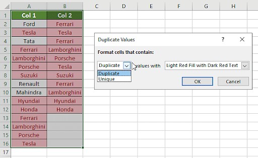
2.1.1. Highlighting Duplicate Values

Select the Columns: Select the range of cells you want to compare.
Go to Conditional Formatting: On the “Home” tab, click “Conditional Formatting” in the “Styles” group.
Highlight Cells Rules: Choose “Highlight Cells Rules” and select “Duplicate Values.”
Choose Formatting: Select the formatting style (e.g., fill color) to highlight duplicate values and click “OK.”

This method highlights all duplicate entries across the selected columns.

2.1.2. Highlighting Unique Values

Select the Columns: Select the range of cells you want to compare.
Go to Conditional Formatting: On the “Home” tab, click “Conditional Formatting” in the “Styles” group.
Highlight Cells Rules: Choose “Highlight Cells Rules” and select “Duplicate Values.”
Change to Unique: In the “Duplicate Values” dialog box, change the selection to “Unique.”
Choose Formatting: Select the formatting style to highlight unique values and click “OK.”

This method highlights all unique entries in the selected columns.

2.1.3. Using Formulas in Conditional Formatting

You can also use formulas to create more complex conditional formatting rules.

Select the Columns: Select the range of cells you want to format.
Go to Conditional Formatting: On the “Home” tab, click “Conditional Formatting” and select “New Rule.”
Use a Formula: Choose “Use a formula to determine which cells to format.”
Enter the Formula: Enter a formula that compares the columns. For example, to highlight cells in column A that match column B, you can use the formula =A1=B1.
Choose Formatting: Click “Format” to select the formatting style and click “OK.”

This method allows you to create custom rules based on specific criteria.

2.2. Using the Equals Operator (=)

The equals operator is a simple way to compare individual cells in two columns.

Create a New Column: Add a new column next to the columns you want to compare.
Enter the Formula: In the first cell of the new column, enter the formula =A1=B1, where A1 and B1 are the first cells in the columns you are comparing.
Drag the Formula: Drag the formula down to apply it to the rest of the rows.

The result will be “TRUE” if the values match and “FALSE” if they don’t.

2.2.1. Customizing Results with the IF Function

You can customize the results using the IF function to display custom messages.

Create a New Column: Add a new column next to the columns you want to compare.
Enter the Formula: In the first cell of the new column, enter the formula =IF(A1=B1, "Match", "No Match"), where A1 and B1 are the first cells in the columns you are comparing.
Drag the Formula: Drag the formula down to apply it to the rest of the rows.

This formula will display “Match” if the values are the same and “No Match” if they are different.

2.3. VLOOKUP Function

The VLOOKUP function is useful for finding matches and extracting corresponding data from another column.

2.3.1. Basic VLOOKUP Formula

The basic syntax for VLOOKUP is:

=VLOOKUP(lookup_value, table_array, col_index_num, [range_lookup])

lookup_value: The value you want to find in the first column of the table_array.
table_array: The range of cells where you want to search.
col_index_num: The column number in the table_array from which to return a value.
[range_lookup]: Optional. TRUE for approximate match, FALSE for exact match.

2.3.2. Using VLOOKUP to Compare Columns

Create a New Column: Add a new column next to the columns you want to compare.
Enter the Formula: In the first cell of the new column, enter the formula =VLOOKUP(A1, B:B, 1, FALSE), where A1 is the first cell in the column you are looking up, and B:B is the column you are searching in.
Handle Errors: Use the IFERROR function to display a custom message when a match is not found. For example, =IFERROR(VLOOKUP(A1, B:B, 1, FALSE), "Not Found").
Drag the Formula: Drag the formula down to apply it to the rest of the rows.

This formula will return the matching value if found, or “Not Found” if not.

2.3.3. Handling Partial Matches with Wildcards

Sometimes, you may need to compare columns with partial matches. You can use wildcards in the VLOOKUP formula to handle these cases.

Create a New Column: Add a new column next to the columns you want to compare.
Enter the Formula: In the first cell of the new column, enter the formula =IFERROR(VLOOKUP("*"&A1&"*", B:B, 1, FALSE), "Not Found").
Drag the Formula: Drag the formula down to apply it to the rest of the rows.

The "*" wildcard allows VLOOKUP to find values that contain the lookup value as a substring.

2.4. IF Function

The IF function is a versatile tool for comparing columns and displaying custom results based on the comparison.

2.4.1. Basic IF Formula

The basic syntax for the IF function is:

=IF(logical_test, value_if_true, value_if_false)

logical_test: The condition you want to test.
value_if_true: The value to return if the condition is true.
value_if_false: The value to return if the condition is false.

2.4.2. Comparing Columns with the IF Function

Create a New Column: Add a new column next to the columns you want to compare.
Enter the Formula: In the first cell of the new column, enter the formula =IF(A1=B1, "Same", "Different"), where A1 and B1 are the first cells in the columns you are comparing.
Drag the Formula: Drag the formula down to apply it to the rest of the rows.

This formula will display “Same” if the values are equal and “Different” if they are not.

2.5. EXACT Function

The EXACT function is used to compare two text strings and returns TRUE if they are exactly the same, including case.

2.5.1. Basic EXACT Formula

The basic syntax for the EXACT function is:

=EXACT(text1, text2)

text1: The first text string.
text2: The second text string.

2.5.2. Comparing Columns with the EXACT Function

Create a New Column: Add a new column next to the columns you want to compare.
Enter the Formula: In the first cell of the new column, enter the formula =EXACT(A1, B1), where A1 and B1 are the first cells in the columns you are comparing.
Drag the Formula: Drag the formula down to apply it to the rest of the rows.

The result will be “TRUE” if the text strings are exactly the same (including case) and “FALSE” if they are not.

3. Advanced Techniques for Column Comparison

For more complex scenarios, you can use advanced techniques to compare columns in Excel.

3.1. Using Array Formulas

Array formulas allow you to perform calculations on multiple values at once.

3.1.1. Comparing Entire Columns

To compare entire columns and return an array of results, you can use an array formula.

Select a Range: Select a range of cells where you want the results to appear. The range should be the same size as the columns you are comparing.
Enter the Formula: Enter the formula =A1:A10=B1:B10, where A1:A10 and B1:B10 are the ranges of cells you are comparing.
Enter as Array Formula: Press Ctrl + Shift + Enter to enter the formula as an array formula.

The result will be an array of TRUE and FALSE values, indicating whether the corresponding cells in the columns are equal.

3.1.2. Counting Matches with Array Formulas

You can use array formulas to count the number of matches between two columns.

Enter the Formula: Enter the formula =SUM(IF(A1:A10=B1:B10, 1, 0)), where A1:A10 and B1:B10 are the ranges of cells you are comparing.
Enter as Array Formula: Press Ctrl + Shift + Enter to enter the formula as an array formula.

The result will be the number of cells where the values in the two columns are equal.

3.2. Using the MATCH Function

The MATCH function returns the position of a value in a range of cells.

3.2.1. Finding Matches in a Column

Create a New Column: Add a new column next to the column you want to search in.
Enter the Formula: In the first cell of the new column, enter the formula =MATCH(A1, B:B, 0), where A1 is the value you want to find, and B:B is the column you are searching in.
Handle Errors: Use the IFERROR function to display a custom message when a match is not found. For example, =IFERROR(MATCH(A1, B:B, 0), "Not Found").
Drag the Formula: Drag the formula down to apply it to the rest of the rows.

This formula will return the row number where the value is found, or “Not Found” if it is not found.

3.3. Combining Functions for Complex Comparisons

You can combine multiple functions to perform more complex column comparisons.

3.3.1. Comparing Columns with Multiple Criteria

For example, you can use the AND function to compare columns based on multiple criteria.

Create a New Column: Add a new column next to the columns you want to compare.
Enter the Formula: In the first cell of the new column, enter the formula =IF(AND(A1>10, B1<20), "Match", "No Match"), where A1 and B1 are the first cells in the columns you are comparing.
Drag the Formula: Drag the formula down to apply it to the rest of the rows.

This formula will display “Match” if the value in column A is greater than 10 and the value in column B is less than 20, and “No Match” otherwise.

4. Practical Scenarios and Examples

Let’s look at some practical scenarios where column comparison in Excel can be applied.

4.1. Data Validation

Scenario: You have two lists of customer IDs, and you want to ensure that all IDs in the first list are also present in the second list.

Use VLOOKUP: Use the VLOOKUP function to search for each ID in the first list in the second list.
Handle Errors: Use the IFERROR function to identify IDs that are not found in the second list.

This helps ensure that your customer data is consistent and accurate.

4.2. Identifying Duplicates

Scenario: You have a list of email addresses, and you want to identify any duplicate entries.

Use Conditional Formatting: Use conditional formatting to highlight duplicate values in the list.
Remove Duplicates: Use the “Remove Duplicates” feature in Excel to remove the duplicate entries.

This helps maintain a clean and accurate email list.

4.3. Comparing Sales Data

Scenario: You have sales data for two different months, and you want to compare the sales figures for each product.

Use the Equals Operator: Use the equals operator to compare the sales figures for each product in the two months.
Use the IF Function: Use the IF function to display whether the sales figures are the same, higher, or lower in the second month.

This helps identify trends and changes in sales performance.

4.4. Comparing Inventory Lists

Scenario: You have two inventory lists, and you want to identify any discrepancies between the lists.

Use VLOOKUP: Use the VLOOKUP function to search for each item in the first list in the second list.
Handle Errors: Use the IFERROR function to identify items that are not found in the second list.
Compare Quantities: Use the IF function to compare the quantities of each item in the two lists.

This helps identify any missing or misplaced items in your inventory.

5. Troubleshooting Common Issues

When comparing columns in Excel, you may encounter some common issues. Here are some tips for troubleshooting:

5.1. Data Type Mismatch

Issue: You are comparing two columns, but the results are not accurate.

Solution: Ensure that the data types in both columns are the same. Use the TYPE function to check the data type of each cell and convert them if necessary.

5.2. Extra Spaces

Issue: You are comparing two text columns, but the results show differences even though the text appears to be the same.

Solution: Remove any extra spaces from the text using the TRIM function. For example, =TRIM(A1) will remove any leading or trailing spaces from the text in cell A1.

5.3. Case Sensitivity

Issue: You are comparing two text columns, and you need to ensure that the comparison is case-sensitive.

Solution: Use the EXACT function to compare the text strings. The EXACT function is case-sensitive and will return TRUE only if the text strings are exactly the same.

5.4. Formula Errors

Issue: You are using a formula to compare columns, but you are getting errors.

Solution: Check the syntax of your formula and ensure that all cell references are correct. Use the IFERROR function to handle any errors and display a custom message.

6. Optimizing Your Excel Worksheets for Column Comparisons

To ensure efficient and accurate column comparisons, optimizing your Excel worksheets is crucial. Here are some best practices:

6.1. Structuring Data for Easy Comparison

Consistent Layout: Ensure that your data is organized in a consistent and logical manner. Use headers for each column to clearly identify the data they contain.
Avoid Merged Cells: Merged cells can cause issues with formulas and data manipulation. Avoid using merged cells in your data range.
Use Tables: Convert your data range into an Excel table (Insert > Table). Tables automatically expand when you add new data, and formulas referencing tables are easier to understand.

6.2. Using Named Ranges

Define Named Ranges: Assign names to your data ranges (Formulas > Define Name). This makes your formulas more readable and easier to maintain.
Refer to Named Ranges in Formulas: Use named ranges in your formulas instead of cell references. For example, if you have a range of sales data named “SalesData”, your formula could be =SUM(SalesData).

6.3. Data Validation

Apply Data Validation Rules: Use data validation to restrict the type of data that can be entered into a cell (Data > Data Validation). This helps prevent errors and inconsistencies in your data.
Create Drop-Down Lists: Use data validation to create drop-down lists for certain columns. This ensures that only valid entries are entered, making column comparisons more accurate.

6.4. Efficient Formula Management

Use Relative and Absolute References: Understand the difference between relative (A1) and absolute ($A$1) cell references. Use absolute references when you want a cell reference to remain constant when copying formulas.
Copy Formulas Efficiently: Use the fill handle (the small square at the bottom-right corner of a cell) to quickly copy formulas down a column.
Check Formulas Regularly: Review your formulas regularly to ensure they are still correct and accurate.

7. Leveraging Excel Add-ins for Advanced Comparisons

Excel add-ins can provide advanced features and capabilities for column comparisons that are not available in the standard Excel installation.

7.1. Power Query

Data Transformation: Power Query (Get & Transform Data in Excel 2010-2016) allows you to import, clean, and transform data from various sources. Use Power Query to combine and compare data from multiple sheets or workbooks.
Column Comparisons: Power Query can perform complex column comparisons and data transformations, such as merging columns, splitting columns, and adding custom columns based on conditional logic.

7.2. ASAP Utilities

Advanced Tools: ASAP Utilities is a popular Excel add-in that provides a wide range of advanced tools and functions.
Compare Data: ASAP Utilities includes features for comparing data in different sheets or workbooks, highlighting differences, and merging data based on matching columns.

7.3. Kutools for Excel

Comprehensive Suite: Kutools for Excel is a comprehensive suite of tools that enhances Excel’s capabilities.
Column Comparison: Kutools provides features for comparing columns, finding differences, and merging data. It also includes tools for advanced formatting and data analysis.

8. FAQs About Comparing Columns in Excel

1. How can I compare two columns and highlight the differences?

Use conditional formatting with a formula. Select the range, go to “Conditional Formatting” > “New Rule”, choose “Use a formula to determine which cells to format”, and enter a formula like =A1<>B1. Then, set the formatting to highlight the differences.

2. What is the best way to compare two columns for exact matches?

Use the EXACT function. Enter the formula =EXACT(A1, B1) in a new column. This function is case-sensitive and returns TRUE if the values are exactly the same, and FALSE otherwise.

3. How do I compare two columns and return a custom message?

Use the IF function. Enter a formula like =IF(A1=B1, "Match", "No Match") in a new column. This will display “Match” if the values are the same and “No Match” if they are different.

4. Can I compare two columns and ignore case?

Yes, use the UPPER or LOWER functions to convert both columns to the same case before comparing. For example, =IF(UPPER(A1)=UPPER(B1), "Match", "No Match").

5. How can I compare two lists and find the matching data?

Use the VLOOKUP function. Enter a formula like =IFERROR(VLOOKUP(A1, B:B, 1, FALSE), "Not Found"). This will search for the value in column A in column B and return the matching value or “Not Found” if there is no match.

6. What is the difference between VLOOKUP and MATCH?

VLOOKUP returns the value from a specified column in a table, while MATCH returns the position of a value in a range. MATCH is often used in combination with INDEX for more flexible lookups.

7. How can I count the number of matches between two columns?

Use an array formula. Enter the formula =SUM(IF(A1:A10=B1:B10, 1, 0)) and press Ctrl + Shift + Enter to enter it as an array formula.

8. How can I compare multiple columns for row matches?

Use the AND function. Enter a formula like =IF(AND(A1=B1, A1=C1), "Complete Match", "No Match"). This will check if all the values in the row are the same.

9. Can I use Power Query to compare columns?

Yes, Power Query can be used to compare columns by merging data, adding custom columns based on conditional logic, and performing various data transformations.

10. Are there any add-ins that can help with column comparisons?

Yes, add-ins like ASAP Utilities and Kutools for Excel provide advanced features for comparing columns, finding differences, and merging data.

9. Taking the Next Steps in Excel Mastery

Mastering column comparisons in Excel is a significant step towards becoming proficient in data analysis and management. However, there’s always more to learn and explore.

9.1. Explore Advanced Excel Functions

INDEX and MATCH: Combine these functions for more flexible and dynamic lookups.
OFFSET: Use OFFSET to create dynamic ranges and perform calculations on changing data sets.
AGGREGATE: Discover the power of AGGREGATE for performing calculations while ignoring errors and hidden rows.

9.2. Dive into Data Visualization

Charts and Graphs: Learn how to create compelling charts and graphs to visualize your data and insights.
PivotTables and PivotCharts: Master PivotTables for summarizing and analyzing large datasets, and use PivotCharts to create interactive visualizations.

9.3. Automate Tasks with Macros

VBA: Explore Visual Basic for Applications (VBA) to automate repetitive tasks and create custom functions in Excel.
Record Macros: Start by recording macros to automate simple tasks and then learn how to edit and customize them using the VBA editor.

9.4. Continue Learning

Online Courses: Enroll in online courses on platforms like Coursera, Udemy, and LinkedIn Learning to expand your Excel knowledge and skills.
Excel Communities: Join Excel communities and forums to connect with other Excel users, ask questions, and share your knowledge.
Microsoft Excel Documentation: Refer to the official Microsoft Excel documentation for detailed information on functions, features, and best practices.

Comparing columns in Excel is a vital skill for anyone working with data. By mastering the techniques and methods discussed in this guide, you can efficiently analyze your data, identify patterns, and make informed decisions. Visit COMPARE.EDU.VN for more in-depth guides and resources to enhance your data analysis capabilities. For any inquiries or further assistance, reach out to us at 333 Comparison Plaza, Choice City, CA 90210, United States, or connect with us on WhatsApp at +1 (626) 555-9090. Explore more at compare.edu.vn and take your data analysis skills to the next level.