Comparing lists in Excel is a crucial skill for data analysis, allowing you to identify matches, differences, and duplicates within your data efficiently. At COMPARE.EDU.VN, we provide detailed comparisons and insights to help you make informed decisions; this guide explores diverse methods to effectively compare lists in Excel using formulas like VLOOKUP, conditional formatting, and other techniques. Learn to analyze your data quickly and accurately for superior data management. Unlock data insights, enhance data validation, and master Excel data comparison through our comprehensive guides.
1. Why Comparing Two Lists in Excel Is Essential
Comparing two lists in Excel is indispensable for various tasks, enhancing data accuracy and decision-making. Here’s why:
- Identifying Missing or Duplicate Entries: Easily spot gaps or repetitions in your data, ensuring completeness and accuracy.
- Validating Records Between Two Databases: Verify data consistency across different sources, crucial for data integrity.
- Analyzing Differences in Datasets: Uncover variations in inventory, sales, or employee datasets, leading to actionable insights.
Excel offers versatile tools to achieve these objectives with ease. At COMPARE.EDU.VN, we understand the importance of efficient data analysis, providing resources and comparisons to optimize your workflows. Contact us at 333 Comparison Plaza, Choice City, CA 90210, United States or via Whatsapp at +1 (626) 555-9090.
2. Five Different Methods to Compare Lists in Excel
Comparing two lists or datasets in Excel helps identify differences, duplicates, or missing entries. This is useful for tasks like data validation or tracking changes. Let’s explore five different methods: using formulas, conditional formatting, and built-in tools to efficiently spot discrepancies. Whether you are comparing data sets, matching data, or trying to identify discrepancies in your data, these methods will help you streamline your data analysis process.
3. Method 1: Using Conditional Formatting to Highlight Differences
Conditional formatting is a simple yet powerful way to compare two lists in Excel. It changes a cell’s appearance based on specific conditions, such as highlighting unique or duplicate values in both lists. This method is particularly useful for visually identifying discrepancies and similarities in your data.
3.1. Step 1: Select Your Data and Go to the Home Tab
Open your Excel spreadsheet, select the data you want to compare, and navigate to the “Home” tab in the Excel ribbon.
3.2. Step 2: Click on Conditional Formatting
In the “Home” tab, click on “Conditional Formatting,” then select “Highlight Cells Rules,” and choose “Duplicate Values.”
.webp)
3.3. Step 3: Select Your Formatting Style
Choose your preferred formatting style from the dropdown list in Excel. Select the formatting tone and press the “OK” button. This will highlight all matching data from the two lists.
3.4. Step 4: Highlight Unique Values
To highlight non-matching data, go to the “Duplicate Values” window and select the “Unique” option. This will highlight all non-matching qualities, making them easy to identify.
.webp)
4. Method 2: Using the Equal Sign Operator for Direct Comparison
The equal sign operator allows you to compare lists cell by cell, returning “TRUE” for matches and “FALSE” for mismatches. This method is straightforward and provides immediate results for each cell comparison. It’s particularly useful for verifying data accuracy row by row.
4.1. Step 1: Insert a New Column
Immediately after the two columns you want to compare, insert a new column. This column will display the results of the comparison.
.webp)
4.2. Step 2: Put the Formula in Cell C2
In cell C2 (or the first cell in your new column), enter the formula =A2=B2. This formula compares the values in cells A2 and B2.
.webp)
4.3. Step 3: Check the Outcome as “TRUE” or “FALSE”
The formula tests whether the value in cell A2 is equal to the value in cell B2. If the cell values match, the outcome will be “TRUE”; if they do not match, the outcome will be “FALSE.”
.webp)
4.4. Step 4: Drag the Formula to Cell C9
Drag the formula down to apply it to the remaining rows. This will determine the results for different qualities and outcomes in each row.
.webp)
Use Case: This method is ideal for comparing data row by row and quickly identifying mismatches.
5. Method 3: Using the VLOOKUP Formula to Find Matches
The VLOOKUP formula is a powerful tool for comparing two lists in Excel, identifying matches or missing values between them. This method is particularly useful when you need to check if values from one list exist in another. It provides a clear indication of whether a match is found or not.
5.1. Step 1: Open Excel and Enter Your Data
Open your MS Excel spreadsheet and enter your lists into the sheet. Ensure your data is organized for easy comparison.
5.2. Step 2: Select a Column for Result
Choose a separate column to display the results of the VLOOKUP formula. This column will indicate whether a match is found or if the value is missing.
5.3. Step 3: Enter VLOOKUP Formula
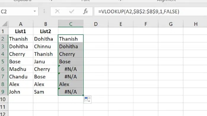
In the first cell of your results column (e.g., C2), enter the following VLOOKUP formula:
=VLOOKUP(A2,$B$2:$B$9,1,FALSE)How VLOOKUP Works:
- A2: The value from List1 to search for.
- $B$2:$B$9: The column range of List2 to look for the value.
- 1: Specifies that you’re searching within the first column of the range.
- FALSE: Ensures an exact match.
5.4. Step 4: Drag the Formula
Drag the fill handle down the results column to apply the formula to all rows. This will perform the VLOOKUP function for each value in List1.
5.5. Step 5: Preview Results
In the results column, whenever a match is found, the name is displayed. If the value from List1 does not exist in List2, the formula will return #N/A. This clearly indicates missing values.
6. Method 4: Using Row Difference to Highlight Discrepancies
The “Row Difference” method allows you to highlight non-matching cells row by line, quickly identifying any discrepancies between two lists. This technique is useful for data validation and ensuring accuracy in your datasets.
6.1. Step 1: Select the Entire Data Range
To highlight non-matching cells row by line, select the entire data range you want to compare. This ensures that the comparison is applied across all relevant cells.
6.2. Step 2: Open ‘Go to Special’ and Press Special Tab
Press the ‘F5’ key to open the ‘Go to special’ box, then click the “Special” tab. This opens the “Go To Special” dialog box, allowing you to select specific cell types.
.webp)
6.3. Step 3: Select ‘Row difference’ and Click OK
In the “Go To Special” window, select the “Row differences” option and click on “OK.” This will highlight all cells that differ from their corresponding cells in each row.
.webp)
6.4. Step 4: Preview Results
The highlighted cells indicate where there is a row difference. You can fill these cells with a color to make the differences stand out even more.
7. Method 5: Using IF Condition to Display Matching or Not Matching Results
Using the IF condition allows you to compare rows in Excel and display results as “Coordinating” or “Not Matching,” providing a clear indication of data consistency. This method is particularly helpful when you need to categorize and label the differences between two lists.
7.1. Step 1: Open Excel Spreadsheet
Open your MS Excel and enter the data you want to compare into the sheet. Organize your data for easy comparison.
7.2. Step 2: Use the Formula
In the first cell of your results column (e.g., C2), enter the following formula:
=IF(A2=B2,"Coordinating","Not Matching")This formula compares the values in cells A2 and B2. If they match, it will display “Coordinating”; if they do not match, it will display “Not Matching.”
.webp)
7.3. Step 3: Apply the Formula to Other Rows
Drag the formula down from the corner of the cell to apply it to other rows (e.g., down to cell C9) to compare additional pairs of values. This will automatically populate the results column with “Coordinating” or “Not Matching” based on the cell comparisons.
.webp)
8. Conclusion: Streamlining Data Comparison in Excel
Comparing two lists or datasets in Excel is an essential skill for data analysis, ensuring data accuracy, and improving efficiency in your workflow. By learning powerful Excel functions like VLOOKUP, MATCH, and advanced tools such as Conditional Formatting and Power Query, you can easily identify matches, discrepancies, and ensure data integrity. Whether you’re handling large Excel databases or comparing data files, these methods provide reliable solutions for your data comparison needs.
Explore more about Excel data comparison and stay ahead with our guides at COMPARE.EDU.VN. Optimize your Excel skills for business intelligence, data validation, and more to boost productivity and achieve precise results. For more information, visit our website or contact us at 333 Comparison Plaza, Choice City, CA 90210, United States. You can also reach us via Whatsapp at +1 (626) 555-9090.
9. Need More Help Comparing Data? Visit COMPARE.EDU.VN Today
Struggling to compare complex datasets or identify discrepancies? COMPARE.EDU.VN offers comprehensive comparisons and expert insights to simplify your data analysis. Whether you need to validate records, analyze differences, or ensure data integrity, our resources provide the solutions you need.
Ready to make data-driven decisions with confidence? Visit compare.edu.vn today and discover the easiest way to compare and analyze your data. Contact us at 333 Comparison Plaza, Choice City, CA 90210, United States or via Whatsapp at +1 (626) 555-9090.
10. Frequently Asked Questions (FAQs) About Comparing Lists in Excel
10.1. How do I compare two lists in Excel to find matches?
To compare two lists in Excel to find matches, you can use the VLOOKUP function. For example, if you have List A in Column A and List B in Column B, you can use the formula =VLOOKUP(A1, B:B, 1, FALSE) in Column C to check for matches. If a match is found, the value from List A will be displayed; otherwise, you’ll get an error.
10.2. How to check if two sets of data match in Excel?
To check if two sets of data match, you can use the IF and COUNTIF functions together. For instance, use =IF(COUNTIF(B:B, A1)>0, “Match”, “No Match”) to see if each value in List A is present in List B. This will return “Match” or “No Match” accordingly.
10.3. How do I compare two Excel databases?
To compare two Excel databases, you can utilize Conditional Formatting. Select the data range in the first database, go to Conditional Formatting > New Rule > Use a formula to determine which cells to format, and enter a formula like =A1<>B1. This will highlight differences between the two databases.
10.4. How do I compare two data files in Excel?
To compare two data files, open both files and use Excel’s View Side by Side feature. Go to the View tab and click “View Side by Side.” You can also use Power Query to load data from both files and merge or compare them using advanced querying capabilities.
10.5. Can I compare lists with different lengths in Excel?
Yes, you can compare lists with different lengths using functions like VLOOKUP or COUNTIF. These functions allow you to check for matches or differences regardless of the list lengths, providing flexibility in your data analysis.
10.6. How can I highlight differences between two lists in Excel?
You can highlight differences between two lists using Conditional Formatting. Use a formula-based rule to compare the values in corresponding cells and apply formatting (e.g., background color) to highlight the differences.
10.7. Is there a way to automate the comparison of two lists in Excel?
Yes, you can automate the comparison of two lists in Excel using macros or Power Query. Macros can automate repetitive tasks, while Power Query allows you to load, transform, and compare data from multiple sources automatically.
10.8. How do I find unique values in two lists in Excel?
To find unique values in two lists, you can combine the lists into a single column and use the “Remove Duplicates” feature. Then, use Conditional Formatting or the COUNTIF function to identify values that appear only once.
10.9. What is the best method for comparing large datasets in Excel?
For comparing large datasets, Power Query is often the best method. It can efficiently load, transform, and compare data from various sources, handling large volumes of data more effectively than traditional Excel formulas.
10.10. How can I ensure data integrity when comparing lists in Excel?
To ensure data integrity, double-check your formulas and data ranges, use absolute references ($) to prevent errors when dragging formulas, and validate your results with manual checks. Additionally, use Excel’s data validation features to enforce data types and formats.