How to Compare Data Using VLOOKUP in Excel

Comparing data across two lists is a common task in Excel. Whether you need to identify matching entries, pinpoint missing information, or retrieve corresponding values, VLOOKUP is a powerful tool. This comprehensive guide will demonstrate various techniques for comparing data using VLOOKUP, equipping you with the skills to efficiently analyze and manage your spreadsheets.

Understanding VLOOKUP for Data Comparison

VLOOKUP (Vertical Lookup) is an Excel function that searches for a specific value in the first column of a table and returns a value in the same row from a specified column. When comparing data, VLOOKUP allows you to determine if a value from one list exists in another.

Basic VLOOKUP Syntax:

=VLOOKUP(lookup_value, table_array, col_index_num, [range_lookup])

lookup_value: The value you want to find.
table_array: The range of cells containing the data you want to search.
col_index_num: The column number in the table_array from which to retrieve a result.
[range_lookup]: Optional. FALSE for an exact match, TRUE for an approximate match. When comparing data, always use FALSE.

Finding Common Values (Matches)

To identify values present in both lists:

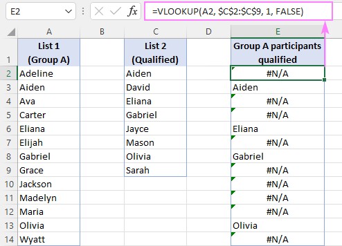
Basic VLOOKUP: Use VLOOKUP to search for each value from the first list in the second list. An exact match (range_lookup = FALSE) will return the found value; otherwise, it returns #N/A.
```
=VLOOKUP(A2, $C$2:$C$9, 1, FALSE)
```
Handling #N/A Errors: Replace #N/A errors with blanks or custom text using IFNA or IFERROR:
```
=IFNA(VLOOKUP(A2, $C$2:$C$9, 1, FALSE), "") 
```
Extracting Only Matches: Filter the results to display only the common values, excluding blanks. In Excel 365, use the FILTER function:
```
 =FILTER(A2:A14, IFNA(VLOOKUP(A2:A14, C2:C9, 1, FALSE), "")<>"")
```

Identifying Missing Values (Differences)

To find values present in the first list but missing in the second:

Detect #N/A Errors: Use ISNA to identify #N/A errors returned by VLOOKUP, indicating missing values.
Return Missing Values: Combine IF and ISNA to return the value from the first list if it’s not found in the second:
```
 =IF(ISNA(VLOOKUP(A2, $C$2:$C$9, 1, FALSE)), A2, "")
```
Dynamic Filtering: In Excel 365, use FILTER with ISNA and VLOOKUP to dynamically extract missing values:
```
 =FILTER(A2:A14, ISNA(VLOOKUP(A2:A14, C2:C9, 1, FALSE)))
```

Comparing Across Different Sheets and Workbooks

To compare data in different sheets or workbooks, adjust the table_array argument in your VLOOKUP formula to include the sheet or workbook name:

=VLOOKUP(A2, Sheet2!$A$2:$A$9, 1, FALSE)

Returning Values from a Third Column

VLOOKUP’s primary function is to retrieve related data. To return a value from a third column based on a match between two other columns:

=VLOOKUP(A3, $D$3:$E$10, 2, FALSE)

Handle #N/A errors as described earlier.

Conclusion

VLOOKUP is a versatile function for comparing data in Excel. By mastering the techniques outlined in this guide, you can effectively identify matches, pinpoint differences, and extract corresponding information, enabling more insightful data analysis and efficient spreadsheet management. Remember to leverage the power of IFNA, IFERROR, and FILTER for cleaner and more dynamic results.