How To Compare Data In Two Excel Sheets Using VLOOKUP

Comparing data in two Excel sheets can be a daunting task. COMPARE.EDU.VN offers a streamlined solution using VLOOKUP, enabling you to reconcile data effectively. This method allows you to identify discrepancies and ensure data accuracy, saving you time and reducing errors. Discover how to utilize Excel formulas and conditional formatting for efficient data comparison, data reconciliation, and error identification.

1. Understanding the Need to Compare Data in Excel

In today’s data-driven world, businesses and individuals often find themselves working with multiple Excel sheets containing similar data. Whether it’s comparing sales figures from different departments, reconciling financial statements, or merging customer lists, the ability to accurately compare data in Excel is crucial. Without a reliable method, you risk making decisions based on incomplete or incorrect information.

1.1. Scenarios Where Data Comparison Is Essential

Consider these common scenarios where comparing data in Excel is vital:

Financial Reconciliation: Accountants like Sara and James at ACME Inc. need to reconcile financial records from different sources to ensure accuracy and identify discrepancies.
Sales Analysis: Sales managers need to compare sales data from different regions or time periods to identify trends and optimize sales strategies.
Inventory Management: Inventory managers need to compare inventory records with physical stock levels to identify discrepancies and prevent stockouts or overstocking.
Customer Relationship Management (CRM): CRM specialists need to compare customer data from different systems to eliminate duplicates and ensure data consistency.
Research and Analysis: Researchers need to compare data from different studies or sources to identify patterns and draw conclusions.

1.2. Challenges of Manual Data Comparison

Manually comparing data in two Excel sheets can be time-consuming, error-prone, and frustrating. Here’s why:

Time Consumption: Manually comparing large datasets can take hours or even days, especially if the data is not well-organized.
Human Error: The risk of human error increases significantly when manually comparing data, leading to inaccurate results.
Lack of Scalability: Manual data comparison is not scalable and becomes impractical as the size and complexity of the data increase.
Difficulty Identifying Discrepancies: It can be challenging to identify subtle differences or discrepancies between two datasets when manually comparing them.
Frustration and Stress: The repetitive and tedious nature of manual data comparison can lead to frustration and stress, impacting productivity and morale.

2. Introducing VLOOKUP: Your Data Comparison Tool

VLOOKUP (Vertical Lookup) is a powerful Excel function that allows you to search for a specific value in a column and return a corresponding value from another column in the same row. It’s particularly useful for comparing data in two Excel sheets because it enables you to quickly find matching values and identify discrepancies.

2.1. What Is VLOOKUP and How Does It Work?

The VLOOKUP function searches for a lookup value in the first column of a table array and returns a value from a specified column in the same row. The syntax of the VLOOKUP function is as follows:

=VLOOKUP(lookup_value, table_array, col_index_num, [range_lookup])

Let’s break down each argument:

lookup_value: The value you want to search for in the first column of the table array.
table_array: The range of cells that contains the data you want to search and retrieve from.
col_index_num: The column number in the table array from which you want to retrieve the matching value.
[range_lookup]: An optional argument that specifies whether you want an exact match (FALSE) or an approximate match (TRUE). For most data comparison tasks, you’ll want to use FALSE to ensure accurate results.

2.2. Advantages of Using VLOOKUP for Data Comparison

Using VLOOKUP for data comparison offers several advantages over manual methods:

Speed and Efficiency: VLOOKUP can quickly compare large datasets, saving you significant time and effort.
Accuracy: VLOOKUP ensures accurate results by finding exact matches based on your specified criteria.
Scalability: VLOOKUP can handle large and complex datasets, making it a scalable solution for data comparison.
Easy Identification of Discrepancies: VLOOKUP makes it easy to identify discrepancies between two datasets by highlighting non-matching values.
Automation: VLOOKUP can be automated using Excel macros, further streamlining the data comparison process.

2.3. Limitations of VLOOKUP

While VLOOKUP is a powerful tool, it’s important to be aware of its limitations:

Lookup Value Must Be in the First Column: VLOOKUP can only search for the lookup value in the first column of the table array.
Case-Insensitive: VLOOKUP is case-insensitive, meaning it doesn’t distinguish between uppercase and lowercase letters.
Error Handling: VLOOKUP returns an error (#N/A) if it can’t find a matching value, which requires error handling to avoid misleading results.
Performance: VLOOKUP can be slow when working with extremely large datasets.
Requires a Common Identifier: VLOOKUP requires a common identifier (e.g., customer ID, invoice number) to match records between the two sheets.

3. Step-by-Step Guide: How to Compare Data Using VLOOKUP

Now that you understand the basics of VLOOKUP, let’s walk through a step-by-step guide on how to use it to compare data in two Excel sheets.

3.1. Step 1: Set Up Your Data in Two Excel Sheets

The first step is to organize your data in two separate Excel sheets. Ensure that both sheets have a common identifier column (e.g., Customer ID, Product Code, Invoice Number) that you can use to match records.

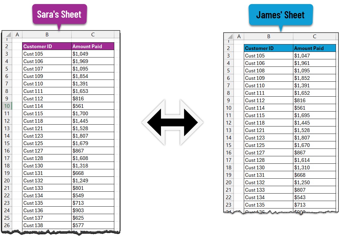
For example, let’s say you have two sheets: “Sara’s Data” and “James’ Data.” Both sheets contain customer payment information, including Customer ID, Customer Name, and Amount Paid. However, the data may not be identical, and you want to compare the two sheets to identify any discrepancies.

3.2. Step 2: Choose the Primary Sheet and Add a VLOOKUP Column

Select one of the sheets as your primary sheet. This is the sheet where you’ll add the VLOOKUP formula to retrieve data from the second sheet. In our example, let’s choose “Sara’s Data” as the primary sheet.

Insert a new column next to the “Amount Paid” column in the primary sheet. This column will contain the VLOOKUP formula. Let’s name this column “James’ Amount Paid.”

3.3. Step 3: Write the VLOOKUP Formula

In the first cell of the “James’ Amount Paid” column (e.g., D2), enter the following VLOOKUP formula:

=VLOOKUP(A2,'James'' Data'!A:B,2,FALSE)

Explanation of the Formula:

A2: This is the lookup value, which is the Customer ID in the current row of the primary sheet (“Sara’s Data”).
'James' Data'!A:B: This is the table array, which is the range of cells in the second sheet (“James’ Data”) that contains the Customer ID and Amount Paid columns.
2: This is the column index number, which specifies that you want to retrieve the value from the second column of the table array (i.e., the “Amount Paid” column in “James’ Data”).
FALSE: This specifies that you want an exact match for the Customer ID.

Alternative using XLOOKUP (if available):

If you have Excel 365 or a later version, you can use the XLOOKUP function, which is more flexible and easier to use than VLOOKUP. The equivalent XLOOKUP formula would be:

=XLOOKUP(A2,'James'' Data'!A:A,'James'' Data'!B:B,"ID Missing")

Explanation of the XLOOKUP Formula:

A2: This is the lookup value, which is the Customer ID in the current row of the primary sheet (“Sara’s Data”).
'James' Data'!A:A: This is the lookup array, which is the range of cells in the second sheet (“James’ Data”) that contains the Customer ID column.
'James' Data'!B:B: This is the return array, which is the range of cells in the second sheet (“James’ Data”) that contains the Amount Paid column.
"ID Missing": This is the value to return if no match is found.

3.4. Step 4: Fill the Formula Down

Once you’ve entered the VLOOKUP formula in the first cell, drag the fill handle (the small square at the bottom right corner of the cell) down to apply the formula to all the rows in the “James’ Amount Paid” column. This will automatically retrieve the corresponding “Amount Paid” values from “James’ Data” for each Customer ID in “Sara’s Data.”

If VLOOKUP can’t find a matching Customer ID in “James’ Data,” it will return the #N/A error. This indicates that the Customer ID is missing in the second sheet.

3.5. Step 5: Reconcile the Values Using the IF Formula

Now that you have the “Amount Paid” values from both sheets in the same row, you can use the IF formula to compare the values and identify any discrepancies.

Insert a new column next to the “James’ Amount Paid” column in the primary sheet. Let’s name this column “Reconciliation Status.”

In the first cell of the “Reconciliation Status” column (e.g., E2), enter the following IF formula:

=IF(ISNA(D2),"ID Missing",IF(D2<>C2,"Not Matching","Matching"))

Explanation of the Formula:

ISNA(D2): This checks if the value in the “James’ Amount Paid” column (D2) is #N/A, which indicates that the Customer ID is missing in “James’ Data.”
"ID Missing": If the Customer ID is missing, the formula returns “ID Missing.”
D2<>C2: This compares the “Amount Paid” value in “James’ Data” (D2) with the “Amount Paid” value in “Sara’s Data” (C2).
"Not Matching": If the values are different, the formula returns “Not Matching.”
"Matching": If the values are the same, the formula returns “Matching.”

Fill the formula down to apply it to all the rows in the “Reconciliation Status” column. This will automatically compare the “Amount Paid” values from both sheets and indicate whether they match, don’t match, or if the Customer ID is missing.

3.6. Step 6: Filter the Data to Identify Discrepancies

Now that you have the “Reconciliation Status” column, you can use Excel’s filtering feature to quickly identify discrepancies between the two sheets.

Select the header row of your data table.
Go to the “Data” tab in the Excel ribbon and click on “Filter.”
Click on the filter arrow in the “Reconciliation Status” column.
Uncheck “Select All” and then check the boxes next to “ID Missing” and “Not Matching.”
Click “OK.”

This will filter the data to show only the rows where the Customer ID is missing in “James’ Data” or where the “Amount Paid” values don’t match between the two sheets. You can then investigate these discrepancies further to determine the cause and take corrective action.

3.7. Step 7: Conditional Formatting for Visual Highlighting (Optional)

To make it even easier to spot discrepancies, you can use Excel’s conditional formatting feature to highlight the “ID Missing” and “Not Matching” records in different colors.

Select the entire range of data (e.g., A1:E100).
Go to the “Home” tab in the Excel ribbon and click on “Conditional Formatting.”
Select “New Rule.”
In the “New Formatting Rule” dialog box, select “Use a formula to determine which cells to format.”
Enter the following formula in the formula box:

=$E2="Not Matching"

Click on the “Format” button and choose a fill color (e.g., red) to highlight the “Not Matching” records.
Click “OK” to close the “Format Cells” dialog box.
Click “OK” to close the “New Formatting Rule” dialog box.
Repeat steps 2-8 to create a second conditional formatting rule for “ID Missing” records, using a different fill color (e.g., yellow). Use the following formula:

=$E2="ID Missing"

Now, all the “Not Matching” records will be highlighted in red, and all the “ID Missing” records will be highlighted in yellow, making it easy to visually identify discrepancies between the two sheets.

4. Advanced Techniques for Data Comparison in Excel

While VLOOKUP is a powerful tool for comparing data in Excel, there are other advanced techniques that you can use to enhance your data comparison capabilities.

4.1. Using INDEX and MATCH as an Alternative to VLOOKUP

The INDEX and MATCH functions can be used together as a more flexible alternative to VLOOKUP. Unlike VLOOKUP, INDEX and MATCH can look up values in any column, not just the first column of the table array.

INDEX Function:

The INDEX function returns the value of a cell in a table based on its row and column number. The syntax of the INDEX function is as follows:

=INDEX(array, row_num, [column_num])

array: The range of cells that contains the data you want to retrieve from.
row_num: The row number in the array from which you want to retrieve the value.
[column_num]: An optional argument that specifies the column number in the array from which you want to retrieve the value.

MATCH Function:

The MATCH function searches for a specified value in a range of cells and returns the relative position of that value in the range. The syntax of the MATCH function is as follows:

=MATCH(lookup_value, lookup_array, [match_type])

lookup_value: The value you want to search for in the lookup array.
lookup_array: The range of cells that contains the data you want to search.
[match_type]: An optional argument that specifies the type of match you want. Use 0 for an exact match.

Using INDEX and MATCH Together:

To use INDEX and MATCH as an alternative to VLOOKUP, you can combine the two functions as follows:

=INDEX('James'' Data'!B:B,MATCH(A2,'James'' Data'!A:A,0))

This formula searches for the Customer ID in cell A2 of the primary sheet (“Sara’s Data”) in the “Customer ID” column of the second sheet (“James’ Data”) and returns the corresponding “Amount Paid” value from the “Amount Paid” column of the second sheet.

4.2. Using Conditional Formatting with Formulas

In addition to using conditional formatting to highlight “ID Missing” and “Not Matching” records, you can also use conditional formatting with formulas to highlight other types of discrepancies, such as:

Values that are above or below a certain threshold: For example, you can highlight “Amount Paid” values that are more than 10% higher or lower than the average.
Duplicate values: You can highlight duplicate Customer IDs or other values that should be unique.
Blank cells: You can highlight blank cells in columns that should contain data.

To use conditional formatting with formulas, follow these steps:

Select the range of cells you want to format.
Go to the “Home” tab in the Excel ribbon and click on “Conditional Formatting.”
Select “New Rule.”
In the “New Formatting Rule” dialog box, select “Use a formula to determine which cells to format.”
Enter the formula in the formula box.
Click on the “Format” button and choose the formatting you want to apply.
Click “OK” to close the “Format Cells” dialog box.
Click “OK” to close the “New Formatting Rule” dialog box.

4.3. Using Power Query for Data Comparison and Transformation

Power Query is a powerful data transformation and analysis tool built into Excel. It allows you to import data from various sources, clean and transform the data, and load it into Excel for analysis. You can use Power Query to compare data from two Excel sheets by merging the data into a single table and then identifying discrepancies.

Here’s a general overview of how to use Power Query for data comparison:

Import Data from Both Sheets: Use Power Query to import the data from both Excel sheets into separate queries.
Add a Custom Column for Source Identification: In each query, add a custom column that identifies the source of the data (e.g., “Sara’s Data” or “James’ Data”).
Append the Queries: Use the “Append Queries” feature to combine the two queries into a single query.
Group and Compare Data: Group the data by the common identifier (e.g., Customer ID) and then use custom columns to compare the values from the different sources.
Load the Results into Excel: Load the transformed data into an Excel sheet for further analysis and reporting.

Power Query is a more advanced technique than VLOOKUP, but it offers greater flexibility and scalability for data comparison, especially when dealing with large and complex datasets.

5. Best Practices for Data Comparison in Excel

To ensure accurate and efficient data comparison in Excel, follow these best practices:

5.1. Ensure Data Consistency

Before comparing data, ensure that the data in both sheets is consistent. This includes:

Data Types: Make sure that the data types are the same in both sheets (e.g., numbers, text, dates).
Formatting: Ensure that the formatting is consistent in both sheets (e.g., currency, decimal places, date formats).
Spelling and Capitalization: Check for spelling errors and inconsistencies in capitalization.
Leading and Trailing Spaces: Remove any leading or trailing spaces from the data.

5.2. Use Unique Identifiers

Use unique identifiers (e.g., Customer ID, Product Code, Invoice Number) to match records between the two sheets. This will ensure that you’re comparing the correct data.

5.3. Handle Missing Values

Decide how you want to handle missing values. You can either:

Ignore them: This will exclude records with missing values from the comparison.
Replace them with a default value: This will allow you to compare records with missing values, but you need to choose a default value that is appropriate for the data.
Flag them: This will identify records with missing values so that you can investigate them further.

5.4. Validate Your Results

After comparing the data, validate your results to ensure that they are accurate. This includes:

Spot-checking: Manually review a sample of the results to ensure that they are correct.
Using formulas to verify the results: Use formulas to calculate summary statistics and compare them to expected values.
Comparing the results to other data sources: Compare the results to other data sources to ensure that they are consistent.

5.5. Document Your Process

Document your data comparison process so that you can easily repeat it in the future. This includes:

Describing the data sources: Describe the data sources that you are comparing.
Explaining the data comparison method: Explain the data comparison method that you are using.
Documenting the formulas and conditional formatting rules: Document the formulas and conditional formatting rules that you are using.
Saving the Excel file with clear and descriptive names: Save the Excel file with clear and descriptive names so that you can easily find it in the future.

6. Automating Data Comparison with Macros

For repetitive data comparison tasks, consider automating the process with Excel macros. Macros are small programs that can automate tasks in Excel, saving you time and effort.

6.1. What Are Excel Macros and How Do They Work?

An Excel macro is a series of commands that you can record and replay to automate a task. Macros are written in Visual Basic for Applications (VBA), a programming language that is built into Excel.

6.2. Benefits of Using Macros for Data Comparison

Using macros for data comparison offers several benefits:

Time Savings: Macros can automate repetitive data comparison tasks, saving you significant time and effort.
Accuracy: Macros can perform data comparison tasks more accurately than humans, reducing the risk of errors.
Consistency: Macros ensure that data comparison tasks are performed consistently every time.
Scalability: Macros can handle large and complex datasets, making them a scalable solution for data comparison.

6.3. Example Macro for Data Comparison

Here’s an example macro that compares data in two Excel sheets using VLOOKUP:

Sub CompareData()

  ' Declare variables
  Dim ws1 As Worksheet, ws2 As Worksheet
  Dim lastRow As Long, i As Long
  Dim lookupValue As Variant, result As Variant

  ' Set worksheet objects
  Set ws1 = ThisWorkbook.Sheets("Sara's Data")
  Set ws2 = ThisWorkbook.Sheets("James' Data")

  ' Find the last row in the primary sheet
  lastRow = ws1.Cells(Rows.Count, "A").End(xlUp).Row

  ' Loop through each row in the primary sheet
  For i = 2 To lastRow ' Assuming data starts from row 2

    ' Get the lookup value from the Customer ID column
    lookupValue = ws1.Cells(i, "A").Value

    ' Use VLOOKUP to find the matching value in the second sheet
    result = Application.WorksheetFunction.VLookup(lookupValue, ws2.Range("A:B"), 2, False)

    ' Check if a match was found
    If IsError(result) Then
      ' If no match was found, write "ID Missing" in the Reconciliation Status column
      ws1.Cells(i, "E").Value = "ID Missing"
    Else
      ' If a match was found, compare the values
      If result <> ws1.Cells(i, "C").Value Then
        ' If the values don't match, write "Not Matching" in the Reconciliation Status column
        ws1.Cells(i, "E").Value = "Not Matching"
      Else
        ' If the values match, write "Matching" in the Reconciliation Status column
        ws1.Cells(i, "E").Value = "Matching"
      End If
    End If

  Next i

  ' Display a message box when the comparison is complete
  MsgBox "Data comparison complete!"

End Sub

Explanation of the Macro:

Declare variables: This section declares the variables that will be used in the macro.
Set worksheet objects: This section sets the worksheet objects for the two sheets that you want to compare.
Find the last row: This section finds the last row in the primary sheet so that the macro knows how many rows to process.
Loop through each row: This section loops through each row in the primary sheet, starting from row 2 (assuming that the data starts from row 2).
Get the lookup value: This section gets the lookup value from the Customer ID column in the current row.
Use VLOOKUP to find the matching value: This section uses the VLOOKUP function to find the matching value in the second sheet.
Check if a match was found: This section checks if a match was found. If no match was found, the macro writes “ID Missing” in the Reconciliation Status column.
Compare the values: If a match was found, this section compares the values in the two sheets. If the values don’t match, the macro writes “Not Matching” in the Reconciliation Status column. If the values match, the macro writes “Matching” in the Reconciliation Status column.
Display a message box: This section displays a message box when the comparison is complete.

To use this macro, follow these steps:

Open the Excel file that contains the data you want to compare.
Press Alt + F11 to open the Visual Basic Editor (VBE).
In the VBE, go to Insert > Module.
Paste the macro code into the module.
Modify the macro code to match your specific data and worksheet names.
Close the VBE.
In Excel, go to the “View” tab and click on “Macros.”
Select the “CompareData” macro and click on “Run.”

The macro will compare the data in the two sheets and write the results in the “Reconciliation Status” column of the primary sheet.

7. Free Comparison & Reconciliation Template

To help you get started with comparing data in Excel, COMPARE.EDU.VN offers a free comparison and reconciliation template. This template includes:

Two sample Excel sheets with customer payment data.
Pre-built VLOOKUP formulas to compare the data.
Conditional formatting rules to highlight discrepancies.
Instructions on how to use the template.

Download the free template here.

8. Other Techniques to Reconcile and Compare Two Excel Sheets

While using VLOOKUP is a quick and elegant way to compare two spreadsheets, Excel also offers few more options. These are:

Using the “Compare and Merge Workbooks” feature: This feature allows you to compare two versions of the same workbook and merge the changes.
Using the “Data > Consolidate” feature: This feature allows you to consolidate data from multiple sheets into a single sheet.
Using third-party Excel add-ins: There are many third-party Excel add-ins that offer advanced data comparison and reconciliation features.

9. COMPARE.EDU.VN: Your Partner in Data Comparison and Decision-Making

At COMPARE.EDU.VN, we understand the challenges of comparing data and making informed decisions. That’s why we provide comprehensive resources and tools to help you compare products, services, and ideas effectively. Whether you’re comparing universities, courses, consumer products, or business solutions, COMPARE.EDU.VN offers objective comparisons and expert insights to empower you to make the right choices.

9.1. Why Choose COMPARE.EDU.VN?

Objective Comparisons: We provide unbiased comparisons based on thorough research and analysis.
Comprehensive Information: We offer detailed information on a wide range of products, services, and ideas.
User Reviews and Ratings: We include user reviews and ratings to provide real-world perspectives.
Expert Insights: We feature expert insights and recommendations to help you make informed decisions.
Easy-to-Use Interface: Our website is designed to be user-friendly and easy to navigate.

9.2. How COMPARE.EDU.VN Can Help You

COMPARE.EDU.VN can help you in various ways:

Save Time and Effort: We do the research for you, saving you time and effort in comparing different options.
Make Informed Decisions: We provide the information you need to make informed decisions based on your specific needs and preferences.
Avoid Costly Mistakes: We help you avoid costly mistakes by providing objective comparisons and expert insights.
Find the Best Solution: We help you find the best solution for your needs, whether it’s a product, service, or idea.

10. Frequently Asked Questions (FAQs)

Here are some frequently asked questions about comparing data in Excel:

Q1: What is the best way to compare data in two Excel sheets?

A: The best way to compare data in two Excel sheets depends on the size and complexity of the data, as well as your specific needs. VLOOKUP is a good option for simple comparisons, while Power Query is a better option for more complex comparisons.

Q2: How do I handle missing values when comparing data in Excel?

A: You can handle missing values by either ignoring them, replacing them with a default value, or flagging them.

Q3: How do I validate my results after comparing data in Excel?

A: You can validate your results by spot-checking, using formulas to verify the results, or comparing the results to other data sources.

Q4: Can I automate data comparison in Excel?

A: Yes, you can automate data comparison in Excel using macros.

Q5: What is the INDEX function in Excel?

A: The INDEX function returns the value of a cell in a table based on its row and column number.

Q6: What is the MATCH function in Excel?

A: The MATCH function searches for a specified value in a range of cells and returns the relative position of that value in the range.

Q7: What is Power Query in Excel?

A: Power Query is a powerful data transformation and analysis tool built into Excel.

Q8: How can I use conditional formatting to highlight discrepancies in Excel?

A: You can use conditional formatting to highlight discrepancies by creating rules that format cells based on specific criteria.

Q9: What are some best practices for data comparison in Excel?

A: Some best practices for data comparison in Excel include ensuring data consistency, using unique identifiers, handling missing values, validating your results, and documenting your process.

Q10: Where can I find more information about data comparison in Excel?

A: You can find more information about data comparison in Excel on the Microsoft website, as well as on various Excel tutorial websites and forums. You can also visit COMPARE.EDU.VN for comprehensive resources and tools for data comparison.

11. Call to Action

Ready to make data-driven decisions with confidence? Visit COMPARE.EDU.VN today to explore our comprehensive comparison tools and resources. Whether you’re evaluating products, services, or ideas, we provide the objective information and expert insights you need to make the right choices.

Take the next step towards informed decision-making:

Browse our comparison categories: COMPARE.EDU.VN
Search for specific products or services: COMPARE.EDU.VN
Contact our experts for personalized guidance: Whatsapp: +1 (626) 555-9090

COMPARE.EDU.VN – Your trusted source for objective comparisons and informed decisions.

Address: 333 Comparison Plaza, Choice City, CA 90210, United States.

In conclusion

Comparing two Excel sheets is an easy task once you know how to use the VLOOKUP (or XLOOKUP) function in Excel. I have used this exact approach countless times when dealing with multiple versions of files or different versions of truth. The process is easy, and the results are actionable. With the guidance provided by compare.edu.vn, you’re well-equipped to streamline your data comparison processes, identify discrepancies with ease, and make informed decisions that drive success.