How to Compare Data in Two Excel Sheets for Matches

Finding matching data across multiple Excel spreadsheets can be a tedious task. Manually comparing rows and columns is time-consuming and prone to errors. Fortunately, Excel offers powerful features to automate this process and quickly identify matches. This guide will explore effective techniques for comparing data in two Excel sheets, focusing on the MATCH function and conditional formatting.

Using the MATCH Function to Find Matches

The MATCH function is a core tool for comparing data in Excel. It searches for a specific value within a range and returns its relative position. This allows you to quickly determine if a value in one sheet exists in another.

1. Prepare Your Data: Ensure both worksheets are in the same workbook.

2. Create a Helper Column: Insert a new column in the sheet where you want to display the match results.

3. Apply the MATCH Formula: In the first cell of the helper column, enter the following formula:

   =MATCH(B2,Sheet1!B2:B6,0)

   • B2: The cell containing the value you want to search for in the other sheet.
   • Sheet1!B2:B6: The range in the other sheet where you want to search.
   • 0: Specifies an exact match.

4. Interpret Results: The formula returns a number indicating the position of the match. If no match is found, it returns #N/A.

Highlighting Matches with Conditional Formatting

Conditional formatting allows you to visually highlight matching data. This makes it easier to identify matches at a glance.

1. Select the Data: Select the column in your sheet where you want to highlight matches.

2. Apply Conditional Formatting: Go to Home > Conditional Formatting > Highlight Cells Rules > Equal To.

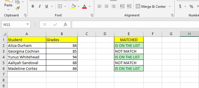
3. Enter the Formula: In the formula box, enter the following:

   =IF(ISNUMBER(MATCH(B2, Sheet1!$B$2:$B$6,0))=TRUE, "IS ON THE LIST", "NOT MATCH")

4. Choose a Formatting Style: Select a formatting style to highlight the matching cells.

5. Review Results: Matching cells will be highlighted based on the chosen formatting.

Combining MATCH with Other Functions

The MATCH function can be combined with other Excel functions like INDEX and VLOOKUP for more advanced data comparison scenarios. For example, INDEX-MATCH allows you to return a value from a specific row and column based on a match.

Conclusion

Comparing data in two Excel sheets for matches is efficiently achieved using the MATCH function and conditional formatting. These techniques enable quick and accurate identification of matching data, significantly improving productivity when working with multiple spreadsheets. Mastering these methods empowers you to streamline data analysis and decision-making processes.