How to Compare Data in Two Excel Sheets: A Step-by-Step Guide

Imagine you are managing data across different departments, or perhaps reconciling financial records from two different quarters. You might find yourself in a situation where you have two Excel sheets containing similar, but potentially different, datasets. Manually comparing these sheets to identify discrepancies or verify matches can be incredibly time-consuming and prone to error. Fortunately, Excel provides powerful tools to streamline this process.

This guide will walk you through a practical, step-by-step method to compare data in two Excel sheets effectively using Excel’s built-in functions like VLOOKUP (or XLOOKUP for newer versions) and IF statements. This approach is perfect for identifying matching records, highlighting discrepancies, and pinpointing missing data between two spreadsheets. Let’s dive in and learn how to efficiently compare your Excel data.

Step 1: Organize Your Data in Excel Sheets

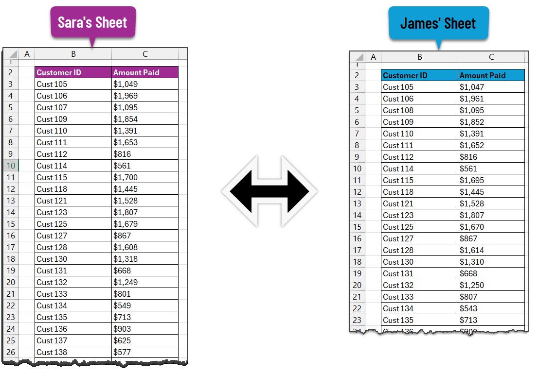
The first step is to ensure your data is clearly organized in two separate sheets within the same Excel workbook. For this example, let’s assume you have two sheets: “Sara’s Data” and “James’ Data”. Both sheets contain customer payment information with identical column headers, but the data entries themselves might vary. It’s crucial that both datasets share a common identifier column, such as “Customer ID” or “Invoice Number,” which will be used as the basis for comparison.

Step 2: Utilizing VLOOKUP to Fetch Matching Data from the Second Sheet

Navigate to the first sheet (“Sara’s Data” in our example). We will now use the VLOOKUP function (or XLOOKUP if you are using Excel 365 or later versions) to bring in corresponding data from the second sheet (“James’ Data”) for each record in the first sheet.

To effectively use VLOOKUP, you need a unique identifier column. In our example, let’s assume “Customer ID” is the unique identifier. We will insert a new column next to your data in the first sheet where the VLOOKUP formula will be placed. This new column will display the “Amount Paid” from the second sheet, matched by “Customer ID”.

Step 3: Applying the VLOOKUP Formula

In the newly created column (for example, column D in “Sara’s Data”), start typing the VLOOKUP formula in the first data row (e.g., cell D3). The formula structure will be as follows:

=VLOOKUP(lookup_value, table_array, col_index_num, [range_lookup])

Using our example, the formula in cell D3 of “Sara’s Data” would be:

=VLOOKUP(B3,'James Sheet'!$B$3:$C$32,2,FALSE)

For XLOOKUP, if you prefer using it, the formula would be:

=XLOOKUP(B3,'James Sheet'!$B$3:$B$32,'James Sheet'!$C$3:$C$32, "ID missing")

Understanding the VLOOKUP Formula:

VLOOKUP: This function searches for a value in the first column of a range and returns a value from a column to the right in the same row.
B3 (lookup_value): This is the “Customer ID” in the current row of “Sara’s Data” (first sheet). VLOOKUP will search for this ID in the second sheet.
'James Sheet'!$B$3:$C$32 (table_array): This specifies the range of data in “James’ Data” (second sheet) where VLOOKUP will search. 'James Sheet!' indicates the sheet name, and $B$3:$C$32 is the data range containing Customer IDs (Column B) and “Amount Paid” (Column C). The $ signs ensure that the range remains fixed when you copy the formula down.
2 (col_index_num): This indicates that we want to retrieve the value from the second column within the table_array range, which is the “Amount Paid” column in “James’ Data”.
FALSE ([range_lookup]): Setting this to FALSE ensures that VLOOKUP looks for an exact match of the “Customer ID”. This is crucial for accurate data comparison.
'James Sheet'!$B$3:$B$32 (lookup_array in XLOOKUP): This is the column containing “Customer IDs” in “James’ Data”.
'James Sheet'!$C$3:$C$32 (return_array in XLOOKUP): This is the column containing “Amount Paid” in “James’ Data”.
"ID missing" ([if_not_found] in XLOOKUP): This is optional and specifies what to display if no match is found.

After entering the formula in cell D3, drag the fill handle (the small square at the bottom-right of the cell) down to apply the formula to all rows in your data.

If a “Customer ID” from “Sara’s Data” is not found in “James’ Data”, VLOOKUP will return a #N/A error. XLOOKUP, if used with the "ID missing" argument, will display “ID missing” instead of #N/A.

Step 4: Reconciling Data with the IF Formula

Now that you have fetched the corresponding “Amount Paid” from “James’ Data” into “Sara’s Data”, you can compare these values to see if they match. We will use the IF formula in another new column (e.g., column E in “Sara’s Data”) to perform this reconciliation.

In cell E3, enter the following IF formula:

=IF(ISERROR(D3),"ID Missing", IF(D3<>C3,"Not matching", "Matching"))

Understanding the IF Formula for Reconciliation:

IF: This function checks a condition and returns one value if the condition is true and another value if false.
ISERROR(D3): This checks if cell D3 (where the VLOOKUP formula is) contains an error value (like #N/A). If it does, it means the “Customer ID” was missing in the second sheet.
"ID Missing": If ISERROR(D3) is true (i.e., ID is missing), the formula returns “ID Missing”.
IF(D3<>C3,"Not matching", "Matching"): If ISERROR(D3) is false (i.e., ID is found), this nested IF formula is executed.
- D3<>C3: This condition checks if the “Amount Paid” from “James’ Data” (in column D) is not equal to the “Amount Paid” in “Sara’s Data” (column C).
- "Not matching": If D3<>C3 is true (amounts are different), the formula returns “Not matching”.
- "Matching": If D3<>C3 is false (amounts are the same), the formula returns “Matching”.

Drag the fill handle down from E3 to apply this formula to all rows. Column E will now clearly indicate whether the data matches, doesn’t match, or if an ID is missing.

You can now use Excel’s filtering capabilities to quickly isolate “Not matching” or “ID Missing” records for further investigation.

Step 5: Visualizing Differences with Conditional Formatting (Optional but Recommended)

To make the discrepancies even more visually apparent, you can use conditional formatting to highlight “Not matching” and “ID Missing” records.

Select Data Range: Select the entire data range in “Sara’s Data” that you want to format (e.g., B3:E32).
Open Conditional Formatting: Go to the “Home” tab on the Excel ribbon, and click on “Conditional Formatting” in the “Styles” group. Select “New Rule”.
Create New Rule: In the “New Formatting Rule” dialog box, choose “Use a formula to determine which cells to format”.
Enter Formula for “Not matching”: In the “Format values where this formula is true” box, enter the formula: =$E3="Not matching" (adjust $E3 to match the first cell in your reconciliation column).
Set Formatting: Click the “Format” button, choose a formatting style (e.g., fill color, font color) to highlight “Not matching” records, and click “OK”.
Add Rule for “ID Missing”: Repeat steps 2-5, but in step 4, use the formula: =$E3="ID Missing" and choose a different formatting style for “ID Missing” records.

With conditional formatting applied, all “Not matching” and “ID Missing” records will be instantly highlighted, making it incredibly easy to identify and address data inconsistencies.

FREE Comparison & Reconciliation Template

For a quicker start, you can download this sample Excel template, pre-configured with the formulas and conditional formatting discussed in this guide.

Beyond VLOOKUP: Alternative Methods for Excel Data Comparison

While VLOOKUP and XLOOKUP offer a straightforward approach, Excel provides other functions and features that can be used for data comparison, depending on your specific needs and data structure. These include:

MATCH and INDEX: These functions, used together, can offer more flexibility than VLOOKUP, particularly when dealing with complex data structures or when you need to retrieve values from columns to the left of the lookup column.
COUNTIF or COUNTIFS: These functions can count the occurrences of specific values or criteria across sheets, useful for quickly identifying duplicates or missing entries based on certain conditions.
Power Query (Get & Transform Data): For more advanced data manipulation and comparison, especially with large datasets or multiple files, Power Query provides robust tools for merging, comparing, and transforming data from various sources, including Excel sheets.

In Conclusion

Comparing data across two Excel sheets doesn’t have to be a daunting task. By leveraging the power of VLOOKUP (or XLOOKUP) and IF formulas, you can efficiently reconcile your data, identify discrepancies, and ensure data accuracy. This step-by-step guide provides a solid foundation for effectively comparing and managing your Excel data, saving you time and improving data integrity. Whether you are reconciling financial statements, comparing sales data, or managing inventory lists, these techniques will empower you to work more efficiently and confidently with your spreadsheets.