How To Compare Columns In Two Excel Files: A Comprehensive Guide

Comparing columns in two Excel files is a common task for data analysts, accountants, and anyone who works with spreadsheets. Whether you’re merging data, identifying discrepancies, or simply ensuring consistency, knowing how to effectively compare columns can save you time and improve accuracy. COMPARE.EDU.VN is here to provide a detailed guide, offering several methods, from simple built-in Excel features to more advanced techniques using formulas and third-party tools. This comprehensive guide will equip you with the knowledge to quickly and accurately compare columns, identify differences, and merge data as needed.

1. Understanding the Need to Compare Columns in Excel

Before diving into the “how,” let’s explore why comparing columns in Excel is a crucial skill. The ability to perform this task efficiently can significantly impact your productivity and the quality of your work. Here are some key scenarios where column comparison is essential:

Data Validation: Ensuring that data entered into one column matches the corresponding data in another column.
Data Integration: Combining data from multiple sources into a unified dataset.
Change Tracking: Identifying modifications made to a column over time.
Error Detection: Pinpointing inconsistencies or errors in data entry.
Report Reconciliation: Verifying that data in different reports aligns correctly.
Auditing: Ensuring compliance with data standards and regulations.
Data Cleansing: Identifying and correcting errors or inconsistencies in data to improve its quality.

2. Simple Visual Comparison: Side-by-Side Viewing

For small datasets, a visual comparison might be sufficient. Excel’s “View Side by Side” feature allows you to display two Excel files or two sheets within the same file simultaneously. This is a quick and easy way to spot obvious differences.

2.1. Comparing Two Excel Workbooks Side by Side

Here’s how to use the “View Side by Side” mode:

Open Both Workbooks: Start by opening the two Excel files you want to compare.
Navigate to the View Tab: In either workbook, go to the “View” tab on the ribbon.
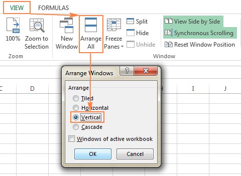
Click “View Side by Side”: In the “Window” group, click the “View Side by Side” button.

By default, Excel displays the windows horizontally. If you prefer a vertical arrangement, click “Arrange All” in the “Window” group and select “Vertical.”

2.2. Synchronous Scrolling

To enhance the visual comparison, enable “Synchronous Scrolling.” This feature ensures that when you scroll in one window, the other window scrolls simultaneously, allowing you to compare rows in parallel.

Ensure Synchronous Scrolling is Enabled: In the “Window” group on the “View” tab, make sure the “Synchronous Scrolling” option is turned on.

2.3. Comparing Two Sheets in the Same Workbook

Sometimes, the columns you want to compare reside in different sheets within the same workbook. Here’s how to view them side by side:

Open the Excel File: Open the workbook containing the two sheets you want to compare.
Create a New Window: Go to the “View” tab and click the “New Window” button in the “Window” group. This opens a second instance of the same workbook.
Enable “View Side by Side”: Click the “View Side by Side” button on the ribbon.
Select the Sheets: In each window, select the sheet you want to compare.

3. Using Excel Formulas for Column Comparison

For more precise comparison, especially with larger datasets, Excel formulas offer a powerful way to identify differences.

3.1. Basic Comparison Formula

The simplest approach is to use an IF statement to compare corresponding cells in two columns.

Open a New Column: In the sheet where you want to display the comparison results, insert a new column next to the columns you are comparing.
Enter the Formula: In the first cell of the new column (e.g., C1), enter the following formula:

=IF(A1=B1, "Match", "Mismatch")
- A1 and B1 are the first cells in the two columns you are comparing.
- "Match" is the text displayed if the cells are identical.
- "Mismatch" is the text displayed if the cells are different.
Copy the Formula Down: Drag the fill handle (the small square at the bottom-right of the cell) down to apply the formula to the rest of the rows.

This formula flags each row as either a “Match” or “Mismatch,” providing a clear indication of where the columns differ.

3.2. Displaying the Differences

Instead of just indicating “Mismatch,” you can modify the formula to display the actual differences.

Modify the Formula: In the comparison column, use the following formula:

=IF(A1=B1, "", A1&" vs "&B1)
- If A1 and B1 are equal, the cell remains empty ("").
- If they are different, the cell displays the values from both cells separated by ” vs “.

This gives you a direct view of the discrepancies between the two columns.

3.3. Handling Errors with `IFERROR`

When comparing columns, you might encounter errors, such as #N/A or #VALUE!, if one column has entries that the other lacks. To handle these errors gracefully, use the IFERROR function.

Wrap the Formula with IFERROR:

=IFERROR(IF(A1=B1, "", A1&" vs "&B1), "Error")
- If the IF statement results in an error, the cell will display “Error” instead of the error code.

This ensures that your comparison column remains clean and readable, even when errors occur.

3.4. Comparing Multiple Criteria

In some cases, you might need to compare columns based on multiple criteria. For example, you might want to ignore case sensitivity or leading/trailing spaces.

3.4.1. Ignoring Case Sensitivity

To ignore case sensitivity, use the UPPER or LOWER functions to convert both cells to the same case before comparing.

Use UPPER or LOWER:

=IF(UPPER(A1)=UPPER(B1), "Match", "Mismatch")

This formula converts both A1 and B1 to uppercase before comparing, effectively ignoring any differences in case.

3.4.2. Removing Leading/Trailing Spaces

To remove leading or trailing spaces, use the TRIM function.

Use TRIM:

=IF(TRIM(A1)=TRIM(B1), "Match", "Mismatch")

This formula removes any leading or trailing spaces from A1 and B1 before comparing.

3.4.3. Combining Multiple Criteria

You can combine these criteria to perform a more robust comparison.

Combine UPPER and TRIM:

=IF(TRIM(UPPER(A1))=TRIM(UPPER(B1)), "Match", "Mismatch")

This formula first trims the spaces and then converts the text to uppercase before comparing.

4. Conditional Formatting for Highlighting Differences

Conditional formatting provides a visual way to highlight differences directly within the columns being compared.

4.1. Highlighting Differences in One Column

To highlight cells in one column that differ from the corresponding cells in another column:

Select the Column: Select the column you want to format (e.g., column A).
Go to Conditional Formatting: On the “Home” tab, in the “Styles” group, click “Conditional Formatting.”
Create a New Rule: Select “New Rule…”
Use a Formula: Choose “Use a formula to determine which cells to format.”
Enter the Formula: In the formula box, enter the following:

=A1<>B1
- This formula checks if the value in cell A1 is different from the value in cell B1.
Format the Cells: Click the “Format…” button, go to the “Fill” tab, and choose a color to highlight the different cells.
Click OK: Click “OK” to apply the rule.

Now, any cell in column A that differs from its corresponding cell in column B will be highlighted.

4.2. Highlighting Differences in Both Columns

To highlight the differences in both columns:

Select Both Columns: Select both columns you want to compare (e.g., columns A and B).
Go to Conditional Formatting: On the “Home” tab, in the “Styles” group, click “Conditional Formatting.”
Create a New Rule: Select “New Rule…”
Use a Formula: Choose “Use a formula to determine which cells to format.”
Enter the Formula: In the formula box, enter the following:

=A1<>B1
- This formula checks if the value in cell A1 is different from the value in cell B1.
Format the Cells: Click the “Format…” button, go to the “Fill” tab, and choose a color to highlight the different cells.
Click OK: Click “OK” to apply the rule.

This highlights differing cells in both columns, making it easy to spot discrepancies.

4.3. Using Different Colors for Added and Removed Entries

To differentiate between added and removed entries, you can use two conditional formatting rules.

For Added Entries (in Column A):
- Select column A.
- Create a new conditional formatting rule using the formula =AND(A1<>"", ISBLANK(B1)).
- Format the cells with one color (e.g., green).
For Removed Entries (in Column B):
- Select column B.
- Create a new conditional formatting rule using the formula =AND(B1<>"", ISBLANK(A1)).
- Format the cells with a different color (e.g., red).

This approach highlights entries that are present in one column but missing in the other, providing a clear visual distinction.

5. Advanced Techniques: Using Excel’s Built-in Features

Excel provides several built-in features that can assist in comparing columns, especially when dealing with structured data.

5.1. Using the `VLOOKUP` Function

The VLOOKUP function can be used to check if values in one column exist in another column and to retrieve corresponding data.

Syntax of VLOOKUP:

=VLOOKUP(lookup_value, table_array, col_index_num, [range_lookup])
- lookup_value: The value you want to search for (e.g., A1).
- table_array: The range in which to search for the value (e.g., B:B).
- col_index_num: The column number in the table_array from which to retrieve a value (use 1 since we are just checking for existence).
- [range_lookup]: FALSE for an exact match.
Example Formula:

=IFERROR(VLOOKUP(A1, B:B, 1, FALSE), "Not Found")
- This formula searches for the value in A1 within column B. If found, it returns the value from column B. If not found, it returns “Not Found.”

This is useful for identifying values in one column that are missing in another.

5.2. Using the `MATCH` Function

The MATCH function returns the position of a value in a range, which can be used to determine if a value exists in another column.

Syntax of MATCH:

=MATCH(lookup_value, lookup_array, [match_type])
- lookup_value: The value you want to search for (e.g., A1).
- lookup_array: The range in which to search for the value (e.g., B:B).
- [match_type]: 0 for an exact match.
Example Formula:

=IFERROR(MATCH(A1, B:B, 0), "Not Found")
- This formula searches for the value in A1 within column B. If found, it returns the row number where the value is located. If not found, it returns “Not Found.”

This is useful for identifying the location of matching values and confirming their existence.

5.3. Using the `COUNTIF` Function

The COUNTIF function counts the number of cells within a range that meet a given criterion. It can be used to check how many times a value from one column appears in another.

Syntax of COUNTIF:

=COUNTIF(range, criterion)
- range: The range in which to count (e.g., B:B).
- criterion: The value to count (e.g., A1).
Example Formula:

=IF(COUNTIF(B:B, A1)>0, "Found", "Not Found")
- This formula counts how many times the value in A1 appears in column B. If the count is greater than 0, it returns “Found”; otherwise, it returns “Not Found.”

This is particularly useful for identifying duplicate entries or verifying the frequency of values across columns.

6. Using Third-Party Tools

While Excel’s built-in features are useful, third-party tools offer more advanced capabilities for comparing columns, especially when dealing with complex datasets or specific comparison requirements.

6.1. Synkronizer Excel Compare

Synkronizer Excel Compare is an add-in designed to compare, merge, and update Excel files and sheets. It offers features such as:

Detailed Difference Reports: Providing comprehensive reports on all types of differences, including values, formulas, and formatting.
Highlighting Differences: Highlighting differences in both sheets for easy identification.
Merging and Updating: Allowing you to transfer individual cells or entire columns/rows between sheets.
Database Comparison: Comparing sheets with a database structure to identify added, deleted, or modified records.

To use Synkronizer Excel Compare:

Install the Add-in: Download and install the Synkronizer Excel Compare add-in.
Open Excel: Open the Excel files you want to compare.
Run Synkronizer: Go to the “Add-ins” tab and click the Synkronizer icon.
Select Workbooks and Sheets: Choose the workbooks and sheets you want to compare.
Configure Comparison Options: Select the comparison options, such as comparing as normal worksheets or as a database.
Start the Comparison: Click the “Start” button to begin the comparison process.
Review the Results: Examine the summary and detailed difference reports to identify discrepancies.

Synkronizer’s advanced features and comprehensive reporting make it a powerful tool for column comparison.

6.2. Ablebits Compare Sheets for Excel

Ablebits Compare Sheets is another add-in that offers a user-friendly interface and robust comparison capabilities. It includes features such as:

Step-by-Step Wizard: Guiding you through the comparison process with a step-by-step wizard.
Comparison Algorithms: Offering different comparison algorithms suited for various data types and structures.
Review Differences Mode: Displaying compared sheets side-by-side in a “Review Differences” mode, allowing you to manage differences one-by-one.
Highlighting Options: Providing options to highlight different types of differences and ignore irrelevant changes.

To use Ablebits Compare Sheets:

Install the Add-in: Download and install the Ablebits Ultimate Suite for Excel, which includes the Compare Sheets tool.
Open Excel: Open the Excel files you want to compare.
Click Compare Sheets: Go to the “Ablebits Data” tab and click the “Compare Sheets” button.
Follow the Wizard: Follow the steps in the wizard to select the sheets, choose the comparison algorithm, and configure the highlighting options.
Compare: Click the “Compare” button to begin the comparison process.
Review Differences: Review the differences in the “Review Differences” mode and merge or ignore changes as needed.

Ablebits Compare Sheets offers a user-friendly approach to column comparison, making it accessible to users of all skill levels.

6.3. xlCompare

xlCompare is a utility designed for comparing and merging Excel files, worksheets, and VBA projects. It provides features such as:

Duplicate Record Detection: Finding and removing duplicate records between worksheets.
Data Updating: Updating existing records in one sheet with values from another sheet.
Merging Capabilities: Adding unique rows and columns from one sheet to another and merging updated records.
Sorting and Filtering: Sorting data by key columns and filtering comparison results.
Highlighting: Highlighting comparison results with colors for easy identification.

xlCompare is a comprehensive tool for managing and comparing Excel data, offering advanced features for data integration and cleansing.

6.4. Change pro for Excel

Change pro for Excel is designed for comparing Excel sheets in both desktop and mobile environments. It offers features such as:

Formula and Value Comparison: Identifying differences in formulas and values between sheets.
Layout Change Detection: Recognizing layout changes, including added and deleted rows and columns.
Embedded Object Recognition: Recognizing embedded objects such as charts, graphs, and images.
Reporting: Creating and printing difference reports of formula, value, and layout differences.
Integration: Comparing files directly from Outlook or document management systems.

Change pro for Excel is a versatile tool for ensuring accuracy and consistency in Excel data across different platforms.

7. Online Services for Column Comparison

In addition to desktop tools, several online services allow you to compare columns without installing any software. While these services may not be suitable for sensitive data, they can be useful for quick comparisons.

7.1. XLComparator

XLComparator is an online service that allows you to upload two Excel files and compare their contents. It highlights differences in the active sheets, providing a quick visual comparison.

7.2. CloudyExcel

CloudyExcel is another online service that allows you to compare Excel files. You upload the files, and the service highlights the differences in the active sheets with different colors.

8. Practical Examples and Scenarios

To illustrate the practical application of these techniques, let’s explore some common scenarios.

8.1. Comparing Sales Data

Imagine you have two Excel files containing sales data from different months. You want to identify which products have increased or decreased in sales.

Open Both Files: Open the two Excel files containing the sales data.
Copy Data to a Single Sheet: Copy the relevant columns (e.g., product name, sales quantity) from both files to a single sheet.
Use Formulas to Compare: Use formulas like IF, VLOOKUP, or COUNTIF to compare the sales quantities for each product.
Apply Conditional Formatting: Use conditional formatting to highlight products with significant increases or decreases in sales.

8.2. Reconciling Bank Statements

You need to reconcile two columns of data, one from the bank statement and the other from internal accounting records.

Copy Data to a Single Sheet: Copy the transaction details from both sources to a single sheet.
Use Formulas to Identify Matches: Use formulas like VLOOKUP or MATCH to identify transactions that appear in both columns.
Highlight Discrepancies: Use conditional formatting to highlight transactions that are missing from either column.
Investigate Discrepancies: Manually investigate the discrepancies to identify and correct any errors.

8.3. Merging Customer Lists

You have two customer lists that you want to merge into a single, comprehensive list.

Copy Data to a Single Sheet: Copy the customer data from both lists to a single sheet.
Remove Duplicates: Use Excel’s “Remove Duplicates” feature to eliminate duplicate entries.
Identify Missing Data: Use formulas like VLOOKUP or COUNTIF to identify customers with missing data in one list.
Fill in Missing Data: Manually fill in the missing data to create a complete customer list.

9. Best Practices for Column Comparison

To ensure accurate and efficient column comparison, follow these best practices:

Clean Your Data: Before comparing columns, clean your data by removing unnecessary spaces, correcting inconsistencies, and standardizing formats.
Use Consistent Formulas: Use consistent formulas throughout your comparison to avoid errors and ensure accurate results.
Test Your Formulas: Test your formulas on a small sample of data before applying them to the entire dataset.
Document Your Process: Document your comparison process, including the formulas used, the steps taken, and any assumptions made.
Back Up Your Data: Before making any changes to your data, back up your original files to avoid data loss.
Use Appropriate Tools: Choose the appropriate tools for your comparison needs, considering the size and complexity of your data.

10. Addressing Common Issues

When comparing columns in Excel, you may encounter some common issues. Here’s how to address them:

Different Data Types: Ensure that the columns you are comparing have the same data types. If not, convert them to a consistent format.
Hidden Rows or Columns: Unhide any hidden rows or columns that may be affecting the comparison results.
Protected Sheets: Unprotect any protected sheets to allow formulas and conditional formatting to work correctly.
Formula Errors: Troubleshoot any formula errors by checking the syntax, cell references, and data types.
Circular References: Avoid circular references, which can cause Excel to recalculate endlessly and produce incorrect results.

11. Automating Column Comparison with VBA

For advanced users, automating column comparison with VBA (Visual Basic for Applications) can save time and effort, especially for repetitive tasks.

11.1. Creating a VBA Macro

To create a VBA macro:

Open the VBA Editor: Press Alt + F11 to open the VBA editor.
Insert a New Module: In the VBA editor, go to “Insert” > “Module.”
Write the VBA Code: Write the VBA code to perform the column comparison.

11.2. Example VBA Code

Here’s an example VBA code to compare two columns and highlight the differences:

Sub CompareColumns()
    Dim ws As Worksheet
    Dim lastRow As Long
    Dim i As Long

    Set ws = ThisWorkbook.Sheets("Sheet1") ' Change "Sheet1" to your sheet name
    lastRow = ws.Cells(Rows.Count, "A").End(xlUp).Row ' Find the last row in column A

    For i = 1 To lastRow
        If ws.Cells(i, "A").Value <> ws.Cells(i, "B").Value Then
            ws.Cells(i, "A").Interior.Color = RGB(255, 0, 0) ' Highlight in red
            ws.Cells(i, "B").Interior.Color = RGB(255, 0, 0) ' Highlight in red
        End If
    Next i

    MsgBox "Comparison complete!"
End Sub

This code compares columns A and B in the specified sheet and highlights the differing cells in red.

11.3. Running the Macro

To run the macro:

Close the VBA Editor: Close the VBA editor and return to Excel.
Run the Macro: Press Alt + F8 to open the “Macro” dialog box.
Select the Macro: Select the “CompareColumns” macro and click “Run.”

This will execute the VBA code and highlight the differences in the specified columns.

12. Conclusion: Empowering Data Analysis with Effective Column Comparison

Comparing columns in two Excel files is a fundamental skill for data analysis, enabling you to validate data, identify discrepancies, and merge information effectively. By mastering the techniques discussed in this guide—from simple visual comparisons and Excel formulas to advanced third-party tools and VBA automation—you can significantly enhance your productivity and ensure the accuracy of your data.

Whether you’re an accountant reconciling financial statements, a data analyst integrating customer lists, or a project manager tracking changes in project data, the ability to compare columns efficiently is invaluable. Embrace these techniques, explore the tools available, and transform your data analysis capabilities.

Ready to take your data analysis skills to the next level? Visit COMPARE.EDU.VN today to discover more comprehensive guides, tool comparisons, and expert insights to help you make the most of your Excel experience.

Need to compare columns in your Excel files and not sure where to start? Don’t struggle alone! Visit COMPARE.EDU.VN for detailed, unbiased comparisons of Excel tools and techniques to help you find the perfect solution for your needs. We provide clear, actionable advice to help you make informed decisions and optimize your data management processes. Check out COMPARE.EDU.VN today and make data comparison easier than ever! Our offices are located at 333 Comparison Plaza, Choice City, CA 90210, United States. For immediate assistance, contact us via Whatsapp: +1 (626) 555-9090, or visit our website at compare.edu.vn.

13. FAQ: Comparing Columns in Excel

Q1: What is the easiest way to compare two columns in Excel?

The easiest way is to use a simple IF formula to check for matches and mismatches between corresponding cells. For example, =IF(A1=B1, "Match", "Mismatch").

Q2: How can I highlight the differences between two columns?

Use conditional formatting with a formula to highlight the differing cells. For example, select the column, go to “Conditional Formatting,” and use the formula =A1<>B1 to highlight cells that are different from their corresponding cells in another column.

Q3: Can I compare columns ignoring case sensitivity?

Yes, use the UPPER or LOWER functions within your formula to convert the text to the same case before comparing. For example, =IF(UPPER(A1)=UPPER(B1), "Match", "Mismatch").

Q4: How do I compare columns and remove leading or trailing spaces?

Use the TRIM function to remove leading or trailing spaces before comparing. For example, =IF(TRIM(A1)=TRIM(B1), "Match", "Mismatch").

Q5: What is the VLOOKUP function used for in column comparison?

The VLOOKUP function is used to check if values in one column exist in another column and retrieve corresponding data. It’s useful for identifying missing values.

Q6: How can I count how many times a value from one column appears in another column?

Use the COUNTIF function. For example, =IF(COUNTIF(B:B, A1)>0, "Found", "Not Found") checks if the value in A1 appears in column B.

Q7: Are there third-party tools for more advanced column comparison?

Yes, tools like Synkronizer Excel Compare, Ablebits Compare Sheets, xlCompare, and Change pro for Excel offer more advanced features such as detailed difference reports, merging capabilities, and database comparison.

Q8: Can I automate the column comparison process?

Yes, you can automate the process using VBA (Visual Basic for Applications). Write a VBA macro to compare the columns and highlight the differences.

Q9: How do I handle errors when comparing columns?

Use the IFERROR function to handle errors gracefully. For example, =IFERROR(IF(A1=B1, "", A1&" vs "&B1), "Error") displays “Error” instead of error codes.

Q10: What should I do before comparing columns to ensure accuracy?

Clean your data by removing unnecessary spaces, correcting inconsistencies, and standardizing formats. Also, back up your data before making any changes.