How to Compare Columns for Duplicates in Excel

Comparing columns for duplicates in Excel can be a time-consuming task, but it’s crucial for data cleansing and analysis. At COMPARE.EDU.VN, we understand the need for efficient solutions, which is why we’ve compiled this comprehensive guide on how to compare columns in Excel to identify and manage duplicate entries. Discover effective methods and techniques to streamline your data analysis process, including conditional formatting, formulas, and more. Master Excel column comparison and ensure data accuracy with these proven techniques.

1. Understanding the Need to Compare Columns in Excel

In the realm of data management and analysis, Microsoft Excel stands as a cornerstone tool. Its versatility allows users to organize, manipulate, and analyze data efficiently. One common task that arises frequently is the need to compare columns for duplicates or discrepancies. This process is essential for data cleansing, ensuring accuracy, and extracting meaningful insights. This is particularly helpful for students, consumers, and professionals across various sectors. Whether you’re comparing product lists, customer databases, or research findings, identifying and addressing differences between columns is crucial for maintaining data integrity.

Imagine a scenario where you’re a marketing analyst comparing sales data from two different quarters. Identifying discrepancies can reveal trends, highlight areas for improvement, and inform strategic decisions. Or perhaps you’re a student comparing research results. Spotting duplicates helps refine your analysis and draw accurate conclusions.

Here, the importance of comparing columns extends beyond mere data handling; it’s about transforming raw information into actionable intelligence. With the right techniques, users can quickly pinpoint variances, eliminate redundant entries, and gain a deeper understanding of their data. This capability empowers individuals and organizations to make informed decisions, optimize processes, and achieve their objectives with confidence. With COMPARE.EDU.VN, comparing data becomes easier than ever.

2. Identifying Search Intent: Why Users Seek Column Comparison Methods

Before diving into the practical methods of comparing columns in Excel, it’s essential to understand the underlying intentions driving users to seek this information. By grasping the specific needs and goals of individuals searching for column comparison techniques, we can tailor our approach to provide the most relevant and effective solutions. Here are five key search intents commonly associated with the query “How To Compare Columns For Duplicates In Excel”:

Finding Duplicates: Users may be searching for a way to identify duplicate entries across multiple columns in Excel. This could be for data cleansing purposes, ensuring accuracy in datasets, or detecting redundant information.
Identifying Unique Values: Conversely, users may seek to identify unique values present in one column but not in another. This is useful for uncovering discrepancies, identifying missing data, or pinpointing differences between datasets.
Comparing Data for Accuracy: Users may want to compare columns to verify the accuracy and consistency of data. This could involve checking for errors, inconsistencies, or discrepancies between related datasets.
Validating Data Integrity: Users may be interested in validating the integrity of data by comparing columns to ensure that it meets certain criteria or standards. This is particularly important in fields such as finance, healthcare, and regulatory compliance.
Streamlining Data Analysis: Ultimately, users may be seeking efficient methods for comparing columns to streamline their data analysis process. By quickly identifying similarities and differences, they can save time, improve productivity, and gain deeper insights from their data.

3. Method 1: Conditional Formatting for Visual Comparison

Conditional formatting in Excel offers a straightforward and visually intuitive method for comparing columns. This technique allows you to highlight duplicate or unique values, making it easy to spot discrepancies at a glance. Here’s how to implement conditional formatting for column comparison:

3.1. Step-by-Step Guide to Conditional Formatting

Select the Columns: Begin by selecting the range of cells in the columns you want to compare. Ensure that you include all relevant data for accurate analysis.
Access Conditional Formatting: Navigate to the “Home” tab on the Excel ribbon. In the “Styles” group, click on “Conditional Formatting” to open the dropdown menu.
Highlight Duplicate Values: From the dropdown menu, choose “Highlight Cells Rules” and then select “Duplicate Values.” This option allows you to format cells containing values that appear more than once in the selected range.
Choose Formatting Options: In the “Duplicate Values” dialog box, you can customize the formatting style for duplicate values. Select a predefined style from the dropdown menu or create a custom format by clicking on “Custom Format.”
Apply Formatting: Once you’ve selected your desired formatting options, click “OK” to apply the conditional formatting rule. Excel will automatically highlight all duplicate values in the selected columns based on your chosen style.

3.2. Benefits of Using Conditional Formatting

Visual Clarity: Conditional formatting provides a clear visual representation of duplicate or unique values, making it easy to identify discrepancies at a glance.
Ease of Use: The conditional formatting feature is user-friendly and requires no complex formulas or coding.
Dynamic Updates: Conditional formatting rules automatically update as you modify the data in your columns, ensuring that the formatting remains accurate and up-to-date.

3.3. Limitations of Conditional Formatting

Limited Customization: While conditional formatting offers some customization options, it may not be suitable for complex comparison scenarios requiring advanced criteria or calculations.
Potential for Misinterpretation: In large datasets, the visual highlighting provided by conditional formatting may become overwhelming or difficult to interpret, especially if there are numerous duplicate values.

4. Method 2: The Equals Operator for Direct Comparison

The equals operator (=) offers a straightforward method for direct comparison of values between two columns in Excel. This technique allows you to quickly identify matching or non-matching entries on a row-by-row basis.

4.1. Step-by-Step Guide to Using the Equals Operator

Create a Result Column: Begin by creating a new column next to the columns you want to compare. This column will display the results of the comparison.
Enter the Formula: In the first cell of the result column, enter the formula =A1=B1, where A1 and B1 are the first cells in the columns you’re comparing. This formula will return TRUE if the values in the two cells are equal and FALSE if they are not.
Drag the Formula: Click and drag the fill handle (the small square at the bottom-right corner of the cell) down to apply the formula to the rest of the rows in the column. Excel will automatically adjust the cell references to compare the corresponding rows.

4.2. Customizing Results with the IF Clause

To display more descriptive results than TRUE and FALSE, you can incorporate the IF clause into your formula. For example, the formula =IF(A1=B1, "Match", "Mismatch") will display “Match” if the values in the two cells are equal and “Mismatch” if they are not.

![IF Clause with Equals Operator](http://compare.edu.vn/wp-content/uploads/2025/04/comparecolumnsinexcel9.jpg){width=494 height=359}
*Alt text: Excel showing results using the IF clause with the equals operator.*

4.3. Advantages of the Equals Operator Method

Simplicity: The equals operator is easy to understand and implement, making it accessible to users of all skill levels.
Direct Comparison: This method provides a direct, row-by-row comparison of values, allowing you to quickly identify discrepancies.
Customizable Results: With the IF clause, you can customize the results to display meaningful messages tailored to your specific needs.

4.4. Limitations of the Equals Operator Method

Case Sensitivity: The equals operator is case-sensitive, meaning that “Apple” and “apple” will be considered different values. If case sensitivity is not desired, consider using the EXACT function.
Exact Matches Only: This method only identifies exact matches between values. It does not account for variations in formatting, spacing, or spelling.

5. Method 3: Leveraging the VLOOKUP Function for Advanced Matching

The VLOOKUP function in Excel offers a powerful and versatile method for comparing columns based on matching values. Unlike the equals operator, VLOOKUP can search for values in one column and return corresponding values from another column, allowing for more complex comparison scenarios.

5.1. Understanding the VLOOKUP Syntax

Before diving into the practical application of VLOOKUP, let’s first understand its syntax:

=VLOOKUP(lookup_value, table_array, col_index_num, [range_lookup])

lookup_value: The value you want to search for in the first column of the table array.
table_array: The range of cells containing the data you want to search.
col_index_num: The column number in the table array from which to return the matching value.
[range_lookup]: An optional argument that specifies whether to find an exact match (FALSE) or an approximate match (TRUE).

5.2. Step-by-Step Guide to Using VLOOKUP for Column Comparison

Create a Result Column: As with the previous method, begin by creating a new column next to the columns you want to compare. This column will display the results of the VLOOKUP function.
Enter the VLOOKUP Formula: In the first cell of the result column, enter the VLOOKUP formula. For example, if you want to search for values from column A in column B and return the corresponding value from column B, the formula would be =VLOOKUP(A1, B:B, 1, FALSE).
Drag the Formula: Click and drag the fill handle down to apply the formula to the rest of the rows in the column. Excel will automatically adjust the cell references to search for corresponding values in each row.

5.3. Handling Errors with IFERROR

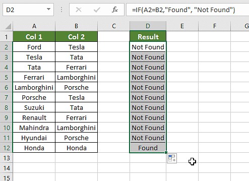
In cases where VLOOKUP cannot find a match, it will return an error (#N/A). To handle these errors and display more meaningful results, you can use the IFERROR function. For example, the formula =IFERROR(VLOOKUP(A1, B:B, 1, FALSE), "Not Found") will display “Not Found” if VLOOKUP cannot find a match for the value in column A.

![Handling error with IFERROR function](http://compare.edu.vn/wp-content/uploads/2025/04/comparecolumnsinexcel13.jpg){width=512 height=367}
*Alt text: Using the IFERROR function to handle errors when no matches are found.*

5.4. Using Wildcards for Partial Matches

In some cases, you may want to compare columns based on partial matches rather than exact matches. For example, you may want to identify values in column A that contain a specific substring from column B. To achieve this, you can use wildcards in conjunction with VLOOKUP. For example, the formula =VLOOKUP("*"&A1&"*", B:B, 1, FALSE) will search for values in column B that contain the value from column A as a substring.

![Using wildcards for partial matches](http://compare.edu.vn/wp-content/uploads/2025/04/comparecolumnsinexcel15.jpg){width=512 height=234}
*Alt text: Demonstrating how to use wildcards for finding partial matches in Excel.*

5.5. Advantages of the VLOOKUP Method

Flexible Matching: VLOOKUP allows for flexible matching based on exact values, partial values, or wildcards.
Error Handling: The IFERROR function enables you to handle errors gracefully and display meaningful results.
Versatility: VLOOKUP can be used for a wide range of comparison scenarios, including finding matching values, extracting corresponding data, and validating data integrity.

5.6. Limitations of the VLOOKUP Method

Limited Search Direction: VLOOKUP can only search for values in the first column of the table array. If you need to search in a different column, you may need to rearrange your data or use a different function.
Performance Considerations: When working with large datasets, VLOOKUP can be computationally intensive and may impact performance.

6. Method 4: Employing the IF Formula for Conditional Outcomes

The IF formula in Excel provides a versatile method for comparing columns and generating conditional outcomes based on the results of the comparison. This technique allows you to define specific criteria for matching or non-matching values and display corresponding messages or perform calculations accordingly.

6.1. Understanding the IF Formula Syntax

Before exploring the practical application of the IF formula, let’s first understand its syntax:

=IF(logical_test, value_if_true, value_if_false)

logical_test: The condition you want to evaluate. This can be a comparison between two values, a logical expression, or a combination thereof.
value_if_true: The value to return if the logical test evaluates to TRUE.
value_if_false: The value to return if the logical test evaluates to FALSE.

6.2. Step-by-Step Guide to Comparing Columns with the IF Formula

Create a Result Column: Begin by creating a new column next to the columns you want to compare. This column will display the results of the IF formula.
Enter the IF Formula: In the first cell of the result column, enter the IF formula. For example, if you want to compare the values in column A and column B and display “Match” if they are equal and “Mismatch” if they are not, the formula would be =IF(A1=B1, "Match", "Mismatch").
Drag the Formula: Click and drag the fill handle down to apply the formula to the rest of the rows in the column. Excel will automatically adjust the cell references to compare the corresponding rows.

6.3. Advantages of the IF Formula Method

Conditional Outcomes: The IF formula allows you to generate conditional outcomes based on the results of the column comparison, providing flexibility and customization.
Clear and Concise: The IF formula is easy to understand and implement, making it accessible to users of all skill levels.
Versatile Applications: The IF formula can be used for a wide range of comparison scenarios, including identifying matching values, flagging discrepancies, and performing calculations based on specific criteria.

6.4. Limitations of the IF Formula Method

Limited Complexity: While the IF formula is suitable for simple comparison scenarios, it may not be sufficient for more complex comparisons requiring multiple criteria or nested conditions.
Potential for Nested Errors: When using nested IF formulas, it’s essential to ensure that all conditions are properly defined to avoid errors or unexpected results.

7. Method 5: Utilizing the EXACT Formula for Case-Sensitive Comparisons

The EXACT formula in Excel offers a specialized method for comparing columns while considering case sensitivity. Unlike the equals operator or the IF formula, EXACT distinguishes between uppercase and lowercase letters, providing a more precise comparison for situations where case matters.

7.1. Understanding the EXACT Formula Syntax

Before delving into the practical application of the EXACT formula, let’s first understand its syntax:

=EXACT(text1, text2)

text1: The first text string to compare.
text2: The second text string to compare.

7.2. Step-by-Step Guide to Comparing Columns with the EXACT Formula

Create a Result Column: Begin by creating a new column next to the columns you want to compare. This column will display the results of the EXACT formula.
Enter the EXACT Formula: In the first cell of the result column, enter the EXACT formula. For example, if you want to compare the values in column A and column B and return TRUE if they are exactly the same (including case) and FALSE if they are not, the formula would be =EXACT(A1, B1).
Drag the Formula: Click and drag the fill handle down to apply the formula to the rest of the rows in the column. Excel will automatically adjust the cell references to compare the corresponding rows.

7.3. Advantages of the EXACT Formula Method

Case-Sensitive Comparisons: The EXACT formula provides a precise comparison that distinguishes between uppercase and lowercase letters, ensuring accuracy when case matters.
Simple and Straightforward: The EXACT formula is easy to understand and implement, making it accessible to users of all skill levels.
Reliable Results: The EXACT formula provides reliable results for case-sensitive comparisons, ensuring that differences are accurately identified.

7.4. Limitations of the EXACT Formula Method

Limited Flexibility: The EXACT formula is limited to comparing two text strings for an exact match. It does not offer options for partial matches or conditional outcomes.
Case Sensitivity Only: The EXACT formula only considers case sensitivity. It does not account for other differences, such as formatting, spacing, or spelling.

8. Choosing the Right Method for Your Scenario

Now that we’ve explored various methods for comparing columns in Excel, it’s essential to understand which method is best suited for different scenarios. Here’s a breakdown to help you choose the right approach:

8.1. Scenario 1: Comparing Two Columns Row-by-Row

In this scenario, you want to compare the values in two columns on a row-by-row basis and identify whether they match or differ. The following formulas are useful:

=IF(A2 = B2, "match", " "): Returns “match” if the values in cells A2 and B2 are equal.
=IF(A2<>B2, "no match", " "): Returns “no match” if the values in cells A2 and B2 are not equal.
=IF(A2 = B2, "match", "no match"): Returns “match” if the values are equal, and “no match” if they differ.

For case-sensitive comparisons, use the following formulas:

=IF(EXACT(A2, B2), "Match", " "): Returns “Match” if the values in cells A2 and B2 are exactly the same, including case.
=IF(EXACT(A2, B2), "Match," "No match"): Returns “Match” if the values are exactly the same, and “No match” if they differ.

8.2. Scenario 2: Comparing Multiple Columns for Row Matches

In this scenario, you want to compare multiple columns and identify rows where all values match. The following formulas are helpful:

=IF(AND(A2=B2, A2=C2), "Complete match", " "): Returns “Complete match” if the values in cells A2, B2, and C2 are all equal.
=IF(COUNTIF($A2:$E2, $A2)=4, "Complete match," "): Returns “Complete match” if there are four occurrences of the value in cell A2 within the range A2:E2.

To compare columns with any two or more cells having the same values in the same row, use these formulas:

=IF(OR(A2=B2, B2=C2, A2=C2), "Match", ""): Returns “Match” if any two of the cells A2, B2, and C2 have the same value.
=IF(COUNTIF(B2:D2,A2)+COUNTIF(C2:D2,B2)+(C2=D2)=0,"Unique","Match"): Returns “Unique” if all values in cells A2, B2, C2, and D2 are unique, and “Match” otherwise.

8.3. Scenario 3: Compare Two Columns for Matches and Differences

In this scenario, you want to compare two datasets and identify the unique values present in one column but not in the other. You can use the following formulas:

=IF(COUNTIF($B:$B, $A2)=0, "Not present in B", ""): Returns “Not present in B” if the value in cell A2 is not found in column B.
=IF(ISERROR(MATCH($A2,$B$2:$B$10,0)),"No present in B",""): Returns “No present in B” if the value in cell A2 is not found in the range B2:B10.

To get the result for both matches and unique values, use this formula:

=IF(COUNTIF($B:$B, $A2)=0, "No Present in B", "Present in B"): Returns “No Present in B” if the value in cell A2 is not found in column B, and “Present in B” otherwise.

8.4. Scenario 4: Compare Two Lists and Pull Matching Data

In this scenario, you want to compare two lists and retrieve matching data from one list based on the values in the other list. The following formulas are useful:

=VLOOKUP(D2, $A$2:$B$6, 2, FALSE): Searches for the value in cell D2 in the range A2:A6 and returns the corresponding value from column B.
=INDEX($B$2:$B$6, MATCH($D2, $A$2:$A$6, 0)): Searches for the value in cell D2 in the range A2:A6 and returns the corresponding value from the range B2:B6.
=XLOOKUP(D2, $A$2:$A$6, $B$2:$B$6): Searches for the value in cell D2 in the range A2:A6 and returns the corresponding value from the range B2:B6.

8.5. Scenario 5: Highlight Row Matches and Differences

In this scenario, you want to highlight rows that include identical values in all columns or highlight the differences in values. You can use conditional formatting with the following formulas:

=AND($A2=$B2, $A2=$C2): Highlights the row if the values in cells A2, B2, and C2 are all equal.
=COUNTIF($A2:$C2, $A2)=3: Highlights the row if there are three occurrences of the value in cell A2 within the range A2:C2.

Alternatively, you can follow these steps to find and highlight matches and differences:

Select the columns you want to compare.
Go to the “Home” tab, click “Find & Select,” and choose “Go To Special.”
Select “Row Differences” and click “OK.”
The cells with different values will be selected. You can then change the fill color to highlight them.

9. Frequently Asked Questions (FAQs)

To further assist you in mastering column comparison in Excel, here are some frequently asked questions along with their answers:

How to compare two columns in Excel?

One popular method for comparing two columns in Excel is to follow these steps: select both columns of data → go to the Home tab → click on Find & Select → choose Go To Special → select Row Differences → click OK.
Is it possible to compare two columns in Excel using the Index-Match function?

Yes, you can compare two columns in Excel using the Index-Match function by creating the required formula for the data required.
How to compare multiple columns in Excel?

To compare multiple columns in Excel, you can use the conditional formatting option on the home and format the setting to “duplicates” or “uniques”, and choose the desired color to highlight the values to compare multiple columns.
How do you compare two lists in Excel for matches?

You can compare two lists in Excel using IF function, MATCH function or highlighting row differences.
How do I compare two columns in Excel and highlight the duplicates?

To compare two columns in Excel and highlight the duplicates, follow these steps:
1. Select the two columns you want to compare.
2. Go to the Home tab and click on Conditional Formatting.
3. Choose “Highlight Cells Rules” and select “Duplicate Values” from the dropdown menu.
4. In the Duplicate Values dialog box, make sure “Duplicate” is selected.
5. Choose a formatting style or leave the default style.
6. Click OK.
Excel will then highlight the duplicate values in the selected columns, making them easy to identify.

10. Take Action: Explore More Comparison Resources at COMPARE.EDU.VN

You’ve now equipped yourself with a comprehensive understanding of how to compare columns for duplicates in Excel using various methods. From conditional formatting to advanced formulas, you have the tools to tackle any data comparison task with confidence.

But why stop here? At COMPARE.EDU.VN, we offer a wealth of resources to further enhance your data analysis skills and decision-making abilities. Whether you’re a student, consumer, or professional, our platform provides objective comparisons and detailed insights to help you make informed choices.

Ready to take your data analysis skills to the next level? Visit COMPARE.EDU.VN today and explore our extensive collection of comparison resources. From product reviews to educational guides, we’ve got everything you need to make smart, data-driven decisions. Your journey to becoming a data analysis expert starts now!

Address: 333 Comparison Plaza, Choice City, CA 90210, United States

WhatsApp: +1 (626) 555-9090

Website: compare.edu.vn