How To Compare Between 2 Columns In Excel

Comparing data in Excel can be a daunting task, especially when dealing with large datasets. But fear not! COMPARE.EDU.VN offers a comprehensive guide on how to compare two columns in Excel, providing you with the knowledge and skills to streamline your data analysis. Unlock hidden patterns, identify discrepancies, and make informed decisions with our easy-to-follow techniques for Excel column comparison.

Are you looking for the best way for column data comparison or data matching? Let’s explore techniques for Excel column analysis.

1. The Importance of Comparing Columns in Excel

Excel is a powerful tool for data storage, manipulation, and analysis. It’s used across various industries for everything from managing finances to tracking sales figures. The ability to compare data within Excel is crucial for several reasons:

• Data Validation: Ensures data accuracy and consistency by identifying discrepancies between different sources.
• Identifying Trends: Uncovers patterns and trends by comparing data over time or across different categories.
• Decision Making: Supports informed decision-making by providing insights based on data comparisons.
• Data Cleaning: Helps identify and correct errors or inconsistencies in datasets.
• Efficiency: Automates the comparison process, saving time and reducing the risk of human error.
• Reporting: Facilitates the creation of clear and concise reports by highlighting key differences and similarities.
• Reconciliation: Simplifies the process of reconciling data from different systems or sources.
• Auditing: Provides a means of auditing data for compliance and accuracy.
• Performance Analysis: Enables performance analysis by comparing actual results against targets or benchmarks.
• Inventory Management: Supports inventory management by comparing stock levels across different locations.

Imagine you’re a marketing manager comparing sales data from two different campaigns to determine which one performed better. Or perhaps you’re an accountant reconciling bank statements with your company’s financial records. In both scenarios, the ability to quickly and accurately compare data in Excel is essential.

Manually comparing columns in large spreadsheets is a time-consuming and error-prone process. Fortunately, Excel offers a range of tools and techniques to automate this process, making it easier to identify matching and mismatching data.
excel compare columns conditional formatting

2. Methods for Comparing Two Columns in Excel

There are several ways to compare two columns in Excel, each with its own strengths and weaknesses. The best method for you will depend on the specific task at hand. Here are some of the most common techniques:

2.1. Using the Equals Operator (=)

This is the simplest method for comparing two columns on a row-by-row basis. You simply enter a formula in a third column that compares the values in the corresponding rows of the two columns you want to compare.

How it Works:

1. In an empty column (e.g., column C), enter the formula =A2=B2 in cell C2. This formula compares the value in cell A2 with the value in cell B2.
2. Press Enter. The formula will return TRUE if the values are the same and FALSE if they are different.
3. Drag the fill handle (the small square at the bottom right of cell C2) down to apply the formula to the rest of the rows in the table.

Example:

Column A (Data 1)	Column B (Data 2)	Column C (Result)
Apple	Apple	TRUE
Banana	Orange	FALSE
Cherry	Cherry	TRUE
Date	Fig	FALSE

Pros:

• Simple and easy to use.
• Provides a clear indication of whether the values in each row match or not.

Cons:

• Only works for exact matches. It’s case-sensitive and doesn’t ignore formatting differences.
• Doesn’t provide any information about the nature of the differences between the columns.
• Can be tedious to analyze the results, especially in large datasets.

2.2. Using the IF Function

The IF function allows you to perform a logical test and return one value if the test is true and another value if the test is false. This can be used to compare two columns and return custom messages based on whether the values match or not.

How it Works:

1. In an empty column (e.g., column C), enter the formula =IF(A2=B2,"Match","Not Match") in cell C2. This formula checks if the value in cell A2 is equal to the value in cell B2. If it is, it returns the message “Match”; otherwise, it returns the message “Not Match”.
2. Press Enter.
3. Drag the fill handle down to apply the formula to the rest of the rows.

Example:

Column A (Data 1)	Column B (Data 2)	Column C (Result)
Apple	Apple	Match
Banana	Orange	Not Match
Cherry	Cherry	Match
Date	Fig	Not Match

Pros:

• More flexible than the equals operator. You can customize the messages that are returned based on the comparison results.
• Still relatively simple to use.

Cons:

• Still only works for exact matches and is case-sensitive.
• Doesn’t provide any information about the nature of the differences between the columns.
• Can be tedious to analyze the results in large datasets.

2.3. Using the EXACT Function

The EXACT function compares two text strings and returns TRUE if they are exactly the same, including case. This is useful when you need to perform a case-sensitive comparison.

How it Works:

1. In an empty column (e.g., column C), enter the formula =IF(EXACT(A2,B2),"Match","Not Match") in cell C2. This formula uses the EXACT function to compare the values in cell A2 and cell B2. If they are exactly the same (including case), it returns the message “Match”; otherwise, it returns the message “Not Match”.
2. Press Enter.
3. Drag the fill handle down to apply the formula to the rest of the rows.

Example:

Column A (Data 1)	Column B (Data 2)	Column C (Result)
Apple	apple	Not Match
Banana	Banana	Match
Cherry	CHERRY	Not Match
Date	Date	Match

Pros:

• Performs a case-sensitive comparison, which is useful in certain situations.

Cons:

• Still only works for exact matches.
• Doesn’t provide any information about the nature of the differences between the columns.
• Can be tedious to analyze the results in large datasets.

2.4. Using Conditional Formatting

Conditional formatting allows you to highlight cells based on certain criteria. This can be used to highlight matching or mismatching values in two columns.

How it Works:

1. Select the range of cells you want to compare (e.g., columns A and B).
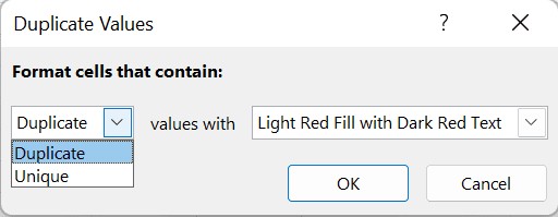
2. Go to Home > Conditional Formatting > Highlight Cells Rules > Duplicate Values.
3. In the Duplicate Values dialog box, choose either Duplicate or Unique from the dropdown menu.
   • Duplicate: Highlights values that appear in both columns.
   • Unique: Highlights values that appear in only one of the columns.
4. Choose a formatting style from the dropdown menu or click Custom Format to create your own.
5. Click OK.

Example:

If you choose Duplicate and select a yellow fill color, all the values that appear in both columns A and B will be highlighted in yellow.

Pros:

• Visually highlights matching or mismatching values, making it easy to identify them.
• Doesn’t require a third column to display the results.

Cons:

• Can be difficult to analyze large datasets with many highlighted cells.
• Doesn’t provide any information about the nature of the differences between the columns.
• Can slow down Excel performance if applied to very large datasets.

2.5. Using the VLOOKUP Function

The VLOOKUP function searches for a value in the first column of a table and returns a value in the same row from another column. This can be used to compare two columns and identify values that are present in one column but not in the other.

How it Works:

1. In an empty column (e.g., column C), enter the formula =VLOOKUP(A2,B:B,1,FALSE) in cell C2. This formula searches for the value in cell A2 in column B. If it finds a match, it returns the value from the same row in column B. If it doesn’t find a match, it returns the error value #N/A.
2. Press Enter.
3. Drag the fill handle down to apply the formula to the rest of the rows.

Example:

Column A (List 1)	Column B (List 2)	Column C (Result)
Apple	Banana	#N/A
Orange	Apple	Apple
Grape	Grape	Grape
Banana	Cherry	#N/A

In this example, the VLOOKUP function searches for each value in column A in column B. If a match is found, the value from column B is returned. If no match is found, the error value #N/A is returned. This allows you to quickly identify values that are present in column A but not in column B.

Pros:

• Can identify values that are present in one column but not in the other.
• Useful for comparing lists and identifying missing items.

Cons:

• Can be slower than other methods, especially for large datasets.
• Requires understanding of the VLOOKUP function and its arguments.
• Only works if the lookup value is in the first column of the lookup range.

2.6. Using the MATCH and INDEX Functions

The MATCH and INDEX functions can be used together to perform more complex comparisons than VLOOKUP. The MATCH function searches for a value in a range of cells and returns the relative position of that value in the range. The INDEX function returns the value of a cell in a table based on its row and column number.

How it Works:

1. In an empty column (e.g., column C), enter the formula =IF(ISNUMBER(MATCH(A2,B:B,0)),"Match","Not Match") in cell C2. This formula uses the MATCH function to search for the value in cell A2 in column B. If a match is found, the MATCH function returns a number (the position of the match). The ISNUMBER function checks if the result of the MATCH function is a number. If it is, the formula returns the message “Match”; otherwise, it returns the message “Not Match”.
2. Press Enter.
3. Drag the fill handle down to apply the formula to the rest of the rows.

Example:

Column A (List 1)	Column B (List 2)	Column C (Result)
Apple	Banana	Not Match
Orange	Apple	Match
Grape	Grape	Match
Banana	Cherry	Not Match

Pros:

• More flexible than VLOOKUP. You can use the MATCH and INDEX functions to perform more complex comparisons.
• Can handle cases where the lookup value is not in the first column of the lookup range.

Cons:

• More complex to use than other methods. Requires a good understanding of the MATCH and INDEX functions.
• Can be slower than other methods, especially for large datasets.

2.7. Using Array Formulas

Array formulas allow you to perform calculations on multiple values at once. This can be used to compare two columns and identify values that are present in one column but not in the other, without using helper columns.

How it Works:

1. Select a range of cells where you want to display the results (e.g., C1:C4 if you have 4 rows of data).
2. Enter the array formula =IF(ISERROR(MATCH(A1:A4,B1:B4,0)),"Not in B","In B").
3. Press Ctrl+Shift+Enter to enter the formula as an array formula. Excel will automatically add curly braces {} around the formula.

Example:

Column A (List 1)	Column B (List 2)	Column C (Result)
Apple	Banana	Not in B
Orange	Apple	In B
Grape	Grape	In B
Banana	Cherry	Not in B

Pros:

• Can perform complex comparisons without using helper columns.
• Can be more efficient than other methods for certain types of comparisons.

Cons:

• More complex to use than other methods. Requires a good understanding of array formulas.
• Can slow down Excel performance if used excessively or on very large datasets.
• Array formulas can be difficult to understand and debug.

3. Advanced Techniques and Considerations

Beyond the basic methods, here are some advanced techniques and considerations for comparing columns in Excel:

• Handling Case Sensitivity: Use the EXACT function for case-sensitive comparisons. For case-insensitive comparisons, you can use the UPPER or LOWER functions to convert the text to the same case before comparing. For example: =IF(UPPER(A2)=UPPER(B2),"Match","Not Match").
• Ignoring Whitespace: Use the TRIM function to remove leading and trailing whitespace from the data before comparing. For example: =IF(TRIM(A2)=TRIM(B2),"Match","Not Match").
• Comparing Numbers with Different Formatting: Use the VALUE function to convert text representations of numbers to numeric values before comparing. This can help avoid issues caused by different formatting. For example: =IF(VALUE(A2)=VALUE(B2),"Match","Not Match").
• Comparing Dates: Ensure that both columns are formatted as dates. You can then use the equals operator or the IF function to compare the dates.
• Using Helper Columns: For complex comparisons, it can be helpful to create helper columns to perform intermediate calculations or transformations. This can make the formulas easier to understand and debug.
• Using Excel Tables: Using Excel tables can make your formulas more robust and easier to maintain. When you use structured references (e.g., Table1[Column1]) in your formulas, Excel automatically adjusts the formulas when you add or remove rows or columns.
• Power Query: For very large datasets or complex data transformations, consider using Power Query (Get & Transform Data) to clean, transform, and compare your data. Power Query is a powerful data manipulation tool that is built into Excel.
• External Tools and Add-ins: There are also a number of third-party Excel add-ins that can help you compare columns and identify differences. These add-ins often provide more advanced features and capabilities than the built-in Excel tools.

4. Real-World Examples

Let’s explore some real-world examples of how you can use these techniques to solve common problems:

4.1. Identifying Duplicate Entries in a Customer List:

Imagine you have two lists of customer names, and you want to identify any duplicate entries. You can use conditional formatting to highlight the duplicate names, or you can use the VLOOKUP function to create a list of names that appear in both lists.

4.2. Comparing Sales Data from Two Different Months:

You want to compare sales data from two different months to see which products performed better in each month. You can use the equals operator or the IF function to compare the sales figures for each product, or you can use conditional formatting to highlight the products that had the biggest increase or decrease in sales.

4.3. Reconciling Bank Statements with Financial Records:

You need to reconcile your bank statements with your company’s financial records. You can use the VLOOKUP function to find matching transactions in both sets of data, and then investigate any transactions that don’t match.

4.4. Verifying Data Accuracy After a Data Migration:

After migrating data from one system to another, you want to verify that the data was migrated correctly. You can use the equals operator, the IF function, or the EXACT function to compare the data in the two systems and identify any discrepancies.

5. Best Practices for Comparing Columns in Excel

To ensure accurate and efficient comparisons, follow these best practices:

• Clean Your Data First: Remove any inconsistencies, errors, or unnecessary formatting from your data before comparing. This may involve removing extra spaces, correcting typos, or standardizing date formats.
• Choose the Right Method: Select the comparison method that is most appropriate for the task at hand. Consider the size of the dataset, the type of data, and the level of detail required.
• Use Clear and Consistent Formulas: Use clear and consistent formulas that are easy to understand and maintain. Avoid using overly complex formulas that are difficult to debug.
• Test Your Formulas: Test your formulas thoroughly to ensure that they are working correctly. Use a small sample of data to verify that the formulas are returning the correct results.
• Document Your Work: Document your work clearly and thoroughly. This will make it easier for you and others to understand and maintain your comparisons in the future.
• Handle Errors Gracefully: Use error handling techniques to prevent errors from crashing your formulas or corrupting your data. The IFERROR function can be used to handle errors gracefully and return a default value if an error occurs.
• Optimize for Performance: For large datasets, optimize your formulas and techniques for performance. Avoid using overly complex formulas or conditional formatting rules that can slow down Excel.
• Use Version Control: Use version control to track changes to your Excel files. This will allow you to easily revert to previous versions if necessary.
• Automate Repetitive Tasks: Use macros or VBA to automate repetitive tasks. This can save you a lot of time and effort, especially if you need to perform the same comparisons on a regular basis.

6. Frequently Asked Questions (FAQ)

Q1: How do I compare two columns in Excel for exact matches?

A: Use the equals operator (=) or the IF function with the equals operator. For example, =IF(A2=B2,"Match","Not Match").

Q2: How do I compare two columns in Excel for case-sensitive matches?

A: Use the EXACT function. For example, =IF(EXACT(A2,B2),"Match","Not Match").

Q3: How do I highlight matching values in two columns?

A: Use conditional formatting with the “Duplicate Values” rule.

Q4: How do I find values that are in one column but not in another?

A: Use the VLOOKUP function or the MATCH and INDEX functions.

Q5: How do I compare two columns in Excel and ignore case?

A: Use the UPPER or LOWER functions to convert the text to the same case before comparing. For example, =IF(UPPER(A2)=UPPER(B2),"Match","Not Match").

Q6: How do I compare two columns in Excel and ignore whitespace?

A: Use the TRIM function to remove leading and trailing whitespace from the data before comparing. For example, =IF(TRIM(A2)=TRIM(B2),"Match","Not Match").

Q7: How do I compare two columns in Excel with different formatting?

A: Use the VALUE function to convert text representations of numbers to numeric values before comparing. For example, =IF(VALUE(A2)=VALUE(B2),"Match","Not Match").

Q8: Can I compare more than two columns at once?

A: Yes, you can compare more than two columns at once by nesting IF functions or using the AND or OR functions. For example, =IF(AND(A2=B2,A2=C2),"Match","Not Match") compares three columns.

Q9: What is the best method for comparing large datasets?

A: For large datasets, consider using Power Query or external tools and add-ins. These tools are designed to handle large amounts of data more efficiently than the built-in Excel functions.

Q10: How do I handle errors when comparing columns in Excel?

A: Use the IFERROR function to handle errors gracefully and return a default value if an error occurs. For example, =IFERROR(VLOOKUP(A2,B:B,1,FALSE),"Not Found").

7. Conclusion: Streamline Your Data Analysis with COMPARE.EDU.VN

Comparing two columns in Excel is a fundamental skill for data analysis. By mastering the techniques and best practices outlined in this guide, you can streamline your data analysis workflow, identify discrepancies, uncover hidden patterns, and make more informed decisions.

Remember to clean your data first, choose the right method for the task at hand, use clear and consistent formulas, test your formulas thoroughly, and document your work clearly.

For more in-depth tutorials, advanced techniques, and real-world examples, visit COMPARE.EDU.VN. We offer a wide range of resources to help you master Excel and other data analysis tools. Whether you’re a beginner or an experienced user, COMPARE.EDU.VN has something to offer you.

Unlock the power of data comparison and make smarter decisions with COMPARE.EDU.VN. Visit our website today at compare.edu.vn or contact us at 333 Comparison Plaza, Choice City, CA 90210, United States. You can also reach us via Whatsapp at +1 (626) 555-9090. Let us help you take your data analysis skills to the next level!