Comparing data in Excel is a common task, whether you’re reconciling invoices, merging customer lists, or analyzing survey results. This tutorial provides a comprehensive guide on how to compare two columns in Excel to identify matching and missing data using various techniques, including VLOOKUP, FILTER, and XLOOKUP. We’ll cover scenarios involving data on the same sheet, different sheets, and even different workbooks.
Using VLOOKUP to Compare Two Columns
VLOOKUP is a powerful function for comparing lists and finding corresponding values. Here’s how to use it to find matches and missing data:
1. Basic VLOOKUP Formula:
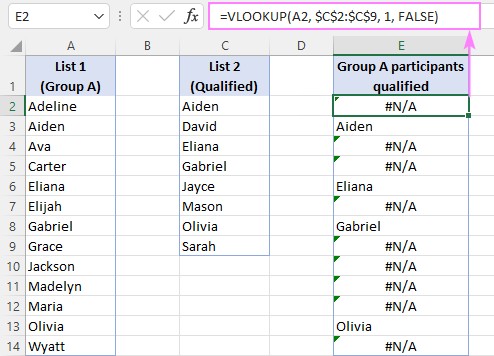
=VLOOKUP(A2, $C$2:$C$9, 1, FALSE)A2: The first cell in the column you want to compare (lookup_value).$C$2:$C$9: The range containing the second column you want to compare (table_array). Use absolute references ($) to ensure the range doesn’t change when copying the formula.1: The column index number within the table_array from which to retrieve a result. Since we’re comparing single columns, this is always 1.FALSE: Specifies an exact match.
This formula searches for the value in A2 within the range C2:C9. If found, it returns the value; otherwise, it returns #N/A, indicating the value is missing in the second column.
2. Handling #N/A Errors:
To replace #N/A errors with blank cells or custom text, use IFNA or IFERROR:
=IFNA(VLOOKUP(A2, $C$2:$C$9, 1, FALSE), "") // Returns blank cell
=IFNA(VLOOKUP(A2, $C$2:$C$9, 1, FALSE), "Not Found") // Returns "Not Found"
Comparing Columns Across Different Sheets and Workbooks
To compare columns on different sheets, use external references:
=IFNA(VLOOKUP(A2, Sheet2!$A$2:$A$9, 1, FALSE), "") Replace “Sheet2” with the actual sheet name. For different workbooks, include the workbook name in square brackets:
=IFNA(VLOOKUP(A2, '[WorkbookName.xlsx]Sheet1'!$A$2:$A$9, 1, FALSE), "")Isolating Matches and Differences
1. Extracting Common Values (Matches):
Use the FILTER function (Excel 365 and later) to dynamically extract matches:
=FILTER(A2:A14, IFNA(VLOOKUP(A2:A14, C2:C9, 1, FALSE), "")<>"")This formula filters the first column, keeping only values that have matches in the second column.
2. Identifying Missing Values (Differences):
To find values present in the first column but missing in the second:
=FILTER(A2:A14, ISNA(VLOOKUP(A2:A14, C2:C9, 1, FALSE)))This filters the first column, keeping only values that result in #N/A errors from the VLOOKUP, indicating they are not found in the second column.
Utilizing XLOOKUP (Excel 365 and later)
XLOOKUP offers a more modern and versatile approach:
Finding Matches:
=FILTER(A2:A14, XLOOKUP(A2:A14, C2:C9, C2:C9,"")<>"")Finding Differences:
=FILTER(A2:A14, XLOOKUP(A2:A14, C2:C9, C2:C9,"")="")XLOOKUP simplifies the formula by handling #N/A errors directly through the optional if_not_found argument.
Conclusion
Excel provides several powerful tools for comparing data and finding missing information. By mastering VLOOKUP, FILTER, and XLOOKUP, you can efficiently analyze and reconcile data sets, saving time and improving accuracy. Choose the method that best suits your specific needs and Excel version. Remember to utilize absolute references and error handling techniques for robust and reliable results.