How to Compare 2 Spreadsheets to Find Matches

Finding matching data across two spreadsheets can be a tedious task if done manually. Fortunately, Excel offers powerful functions to automate and simplify this process. This guide provides a step-by-step approach on how to compare two Excel sheets for matching data within the same workbook using the MATCH and IF functions, along with conditional formatting for easy visualization.

Using the MATCH Function to Find Matches

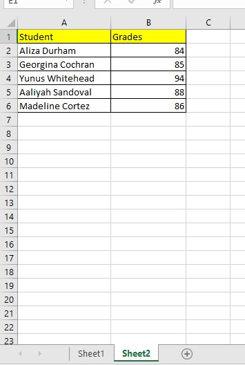
The MATCH function returns the relative position of a matching value within a range. Here’s how to use it for comparing two spreadsheets:

1. Prepare your data: Ensure both worksheets are within the same Excel workbook.
2. Create a helper column: In the sheet where you want to display the results, insert a new column.
3. Enter the formula: In the first cell of the helper column, enter the following formula: =MATCH(B2,Sheet1!B2:B6,0). Replace B2 with the cell containing the value you want to search for, Sheet1 with the name of the sheet you’re comparing against, and B2:B6 with the range containing the data you want to search within. The 0 in the formula ensures an exact match.
4. Interpret the results: The formula returns a number indicating the position of the match. If no match is found, it returns #N/A.

Highlighting Matches with Conditional Formatting

For a visual representation of the matches, use conditional formatting:

1. Select the data: Select the column in your main sheet where you want to highlight matches.
2. Apply conditional formatting: Go to Home > Conditional Formatting > Highlight Cells Rules > Equal To.
3. Enter the criteria: In the dialog box, select “IS ON THE LIST” (you’ll define this in the next step using the IF function) and choose a formatting style to highlight the matching cells.
4. Use the IF Function: Before finalizing the conditional formatting, you need to create a separate column and use the IF function combined with MATCH to determine if a value is present in the other sheet. Use this formula: =IF(ISNUMBER(MATCH(B2,Sheet1!$B$2:$B$6,0))=TRUE,"IS ON THE LIST","NOT MATCH"). This formula checks if the MATCH function returns a number (indicating a match) and displays “IS ON THE LIST” if true, and “NOT MATCH” otherwise.
5. Finalize Conditional Formatting: Now you can go back to step 3 and finalize it. Excel will highlight cells containing “IS ON THE LIST.”

Utilizing VLOOKUP for Comparing Spreadsheets

While MATCH and IF provide a robust solution, VLOOKUP can also be employed. By assigning range names to your data in each sheet, you can use VLOOKUP to search for specific values and retrieve corresponding data from the other spreadsheet. This is particularly helpful if you need to extract more information than just the position of the match.

Conclusion

Comparing two spreadsheets to find matches is a common task made easy with Excel’s built-in functions. The MATCH function pinpoints the location of matching data, while conditional formatting provides a clear visual representation. By combining these techniques, you can efficiently analyze and compare data across multiple spreadsheets, saving time and improving accuracy. Using VLOOKUP adds another layer of flexibility, allowing you to retrieve associated information from the matching rows. Choose the method that best suits your needs and data structure for optimal results.