Comparing data in Excel is a common task, especially when dealing with large datasets. This article provides a comprehensive guide on how to compare two Excel columns for differences, utilizing various techniques, from simple formulas to advanced tools. We’ll cover methods for finding exact matches, case-sensitive matches, and highlighting discrepancies.
Comparing Two Columns Row-by-Row for Matches and Differences
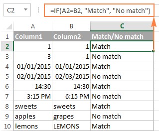
The simplest way to compare two Excel columns row-by-row is using the IF function. Let’s explore different scenarios:
Finding Exact Matches
To identify matching cells in the same row (e.g., A2 and B2), use this formula:
=IF(A2=B2,"Match","")This formula compares the values in A2 and B2. If they are identical, it returns “Match”; otherwise, it returns an empty string.
Finding Differences
To pinpoint differences between cells in the same row, use the not-equal-to operator:
=IF(A2<>B2,"No match","")This formula returns “No match” if the values in A2 and B2 differ; otherwise, it returns an empty string.
Identifying Both Matches and Differences
You can combine the above formulas to display both matches and differences:
=IF(A2=B2,"Match","No match")Case-Sensitive Comparison
For case-sensitive matching, utilize the EXACT function:
=IF(EXACT(A2, B2), "Match", "Unique")This formula returns “Match” only if the values in A2 and B2 are identical, including case. Otherwise, it returns “Unique”.
Comparing Multiple Columns for Matches in the Same Row
You can extend these comparisons to multiple columns:
Finding Matches Across All Columns
To find rows with identical values across all columns (e.g., A2, B2, and C2), use the AND function:
=IF(AND(A2=B2, A2=C2), "Full match", "")For a larger number of columns, the COUNTIF function offers a more efficient solution:
=IF(COUNTIF($A2:$E2, $A2)=5, "Full match", "")Where ‘5’ represents the number of columns being compared.
Finding Matches in Any Two Cells within the Same Row
To find rows where at least two cells match, use the OR function:
=IF(OR(A2=B2, B2=C2, A2=C2), "Match", "")For numerous columns, a combination of COUNTIF functions provides a more manageable approach.
Comparing Two Columns for Matches and Highlighting Differences
To visually identify differences between two columns, leverage Excel’s Conditional Formatting:
Highlighting Matches in the Same Row
- Select the cells you want to format.
- Go to Conditional Formatting > New Rule… > Use a formula to determine which cells to format.
- Enter the formula
=$B2=$A2(assuming data starts in row 2).
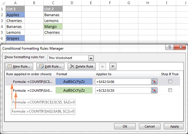
Highlighting Unique Entries
To highlight entries present in one column but not the other, use COUNTIF within Conditional Formatting. For example, to highlight unique values in column A:
=COUNTIF($C$2:$C$5, $A2)=0
``` {width=636 height=456}
## Comparing Two Lists and Extracting Matches
Beyond simply identifying matches and differences, you might need to extract matching data. Functions like VLOOKUP, INDEX MATCH, and XLOOKUP (in Excel 2021 and 365) can help achieve this.
```excel
=VLOOKUP(D2, $A$2:$B$6, 2, FALSE)Formula-Free Comparison Methods
For those less comfortable with formulas, third-party add-ins like “Compare Two Tables” offer a user-friendly interface to compare and highlight differences between datasets.
This comprehensive guide provides a solid foundation for comparing two Excel columns for differences. Choose the method best suited to your specific needs and data structure. Remember to adjust formulas and ranges to match your actual data.