How To Compare 2 Columns Of Data In Excel

Comparing two columns of data in Excel is crucial for data analysis, cleaning, and reporting. This article from COMPARE.EDU.VN provides a comprehensive guide on comparing columns in Excel, offering various methods and techniques to suit different scenarios. Learn effective ways to perform column comparisons, identify differences, and ensure data integrity using Excel’s powerful features.

1. Understanding the Basics of Comparing Columns in Excel

Comparing columns in Excel involves checking corresponding cells in two or more columns to identify similarities, differences, or patterns. This process is essential for various tasks, including:

• Data Validation: Ensuring data consistency and accuracy by comparing columns for discrepancies.
• Data Cleaning: Identifying and correcting errors or inconsistencies between columns.
• Data Analysis: Extracting insights by comparing different data sets.
• Reporting: Highlighting key differences and similarities in reports.

Excel offers several methods for comparing columns, ranging from simple formulas to advanced features like conditional formatting and the VLOOKUP function. The choice of method depends on the specific requirements of the comparison and the size of the data set.

2. Methods for Comparing Two Columns in Excel

2.1. Conditional Formatting

Conditional formatting is a quick and visual way to compare two columns in Excel. It allows you to highlight cells that meet specific criteria, such as matching or unique values.

Steps:

1. Select the two columns you want to compare.
2. Go to the Home tab and click on Conditional Formatting.
3. Choose Highlight Cells Rules.
4. Select Duplicate Values or Unique Values to highlight matching or unique entries, respectively.

Benefits:

• Easy and quick to set up.
• Visually highlights differences and similarities.
• No formulas required.

Limitations:

• Limited to highlighting based on simple criteria (duplicates or uniques).
• Does not provide detailed information about the differences.

2.2. Using the Equals Operator (=)

The equals operator is a simple formula-based method for comparing two columns in Excel. It returns TRUE if the values in the corresponding cells are the same, and FALSE otherwise.

Formula:

=A1=B1

Where A1 and B1 are the first cells in the two columns you want to compare.

Steps:

1. Create a new column to display the comparison results.
2. Enter the formula in the first cell of the new column, referencing the corresponding cells in the two columns you want to compare.
3. Drag the formula down to apply it to all rows.

Benefits:

• Simple and straightforward.
• Provides a clear TRUE/FALSE result for each row.

Limitations:

• Only indicates whether the values are the same or different, without providing additional details.
• Case-sensitive, meaning “Apple” and “apple” will be considered different.

2.3. The IF Formula

The IF formula allows you to display custom messages based on whether the values in two columns are the same or different. This method provides more flexibility than the equals operator.

Formula:

=IF(A1=B1, "Match", "No Match")

Where A1 and B1 are the first cells in the two columns you want to compare.

Steps:

1. Create a new column to display the comparison results.
2. Enter the formula in the first cell of the new column, referencing the corresponding cells in the two columns you want to compare.
3. Drag the formula down to apply it to all rows.

Benefits:

• Allows for custom messages to indicate matches and differences.
• More informative than the equals operator.

Limitations:

• Still case-sensitive.
• Only provides a basic “match” or “no match” result.

2.4. The EXACT Formula

The EXACT formula is similar to the equals operator and the IF formula, but it is case-sensitive. It returns TRUE only if the values in the corresponding cells are exactly the same, including case.

Formula:

=EXACT(A1, B1)

Where A1 and B1 are the first cells in the two columns you want to compare.

Steps:

1. Create a new column to display the comparison results.
2. Enter the formula in the first cell of the new column, referencing the corresponding cells in the two columns you want to compare.
3. Drag the formula down to apply it to all rows.

Benefits:

• Ensures accurate comparisons when case sensitivity is important.

Limitations:

• Can be too strict in situations where case differences are not significant.

2.5. The VLOOKUP Function

The VLOOKUP function is a powerful tool for comparing two columns and identifying values that exist in one column but not in the other. It searches for a value in the first column and returns a corresponding value from another column.

Formula:

=VLOOKUP(A1, B:B, 1, FALSE)

Where A1 is the value you want to search for, B:B is the range of cells in the second column, 1 is the column index number (in this case, the first column in the range), and FALSE specifies an exact match.

Steps:

1. Create a new column to display the comparison results.
2. Enter the formula in the first cell of the new column, referencing the cell in the first column and the range of cells in the second column.
3. Drag the formula down to apply it to all rows.
4. If the value in the first column is found in the second column, VLOOKUP will return the matching value. If the value is not found, it will return an error (#N/A).
5. You can use the IFERROR function to replace the error with a custom message.

Modified Formula:

=IFERROR(VLOOKUP(A1, B:B, 1, FALSE), "Not Found")

Benefits:

• Identifies values that exist in one column but not in the other.
• Can return corresponding values from the second column.
• Handles errors gracefully with the IFERROR function.

Limitations:

• More complex than other methods.
• Can be slower for large data sets.

3. Comparing Multiple Columns in Excel

In addition to comparing two columns, Excel also provides methods for comparing multiple columns simultaneously. This is useful when you need to identify rows where all values match or where there are any differences.

3.1. Using the AND Function

The AND function allows you to check if multiple conditions are true. You can use it to compare multiple columns and identify rows where all values are the same.

Formula:

=IF(AND(A1=B1, A1=C1, A1=D1), "Match", "No Match")

Where A1, B1, C1, and D1 are the first cells in the columns you want to compare.

Steps:

1. Create a new column to display the comparison results.
2. Enter the formula in the first cell of the new column, referencing the corresponding cells in the columns you want to compare.
3. Drag the formula down to apply it to all rows.

Benefits:

• Identifies rows where all values match across multiple columns.

Limitations:

• Becomes cumbersome with a large number of columns.
• Only indicates whether all values match or not, without providing details about the differences.

3.2. Using the COUNTIF Function

The COUNTIF function counts the number of cells within a range that meet a given criteria. You can use it to compare multiple columns and identify rows where all values are the same.

Formula:

=IF(COUNTIF(A1:D1, A1)=4, "Match", "No Match")

Where A1:D1 is the range of cells you want to compare, and 4 is the number of columns in the range.

Steps:

1. Create a new column to display the comparison results.
2. Enter the formula in the first cell of the new column, referencing the range of cells you want to compare.
3. Drag the formula down to apply it to all rows.

Benefits:

• More concise than the AND function for comparing a large number of columns.

Limitations:

• Only indicates whether all values match or not.

3.3. Conditional Formatting with Formulas

You can use conditional formatting with formulas to highlight rows where all values match or where there are any differences.

Steps:

1. Select the range of cells you want to compare.
2. Go to the Home tab and click on Conditional Formatting.
3. Choose New Rule.
4. Select Use a formula to determine which cells to format.
5. Enter a formula to check if all values match or if there are any differences.
6. Choose a formatting style to highlight the cells that meet the criteria.

Example Formula for Highlighting Rows Where All Values Match:

=COUNTIF($A1:$D1, $A1)=4

Benefits:

• Provides visual cues for identifying matches and differences across multiple columns.

Limitations:

• Requires some knowledge of Excel formulas.

4. Advanced Techniques for Column Comparison

4.1. Using Array Formulas

Array formulas allow you to perform complex calculations on ranges of cells. You can use them to compare columns and identify specific differences or patterns.

Example:

To find the number of differences between two columns, you can use the following array formula:

=SUM(IF(A1:A10<>B1:B10, 1, 0))

This formula compares each cell in the range A1:A10 with the corresponding cell in the range B1:B10 and returns 1 if they are different and 0 if they are the same. The SUM function then adds up all the 1s to give you the total number of differences.

Note: To enter an array formula, you need to press Ctrl+Shift+Enter.

Benefits:

• Allows for complex comparisons and calculations.

Limitations:

• Can be difficult to understand and use.
• Can slow down performance for large data sets.

4.2. Using Power Query

Power Query is a powerful data transformation and analysis tool that is built into Excel. You can use it to compare columns, merge data from multiple sources, and perform other advanced data manipulation tasks.

Steps:

1. Select the data range of the first column and go to Data > From Table/Range.
2. In the Power Query Editor, rename the query to something descriptive.
3. Repeat the process for the second column.
4. Go to Home > Merge Queries.
5. Select the two queries you created and choose the column to compare.
6. Choose the join kind (e.g., Left Outer, Right Outer, Full Outer) to specify which rows to include in the result.
7. Expand the merged column to include the columns from the second query.
8. Compare the columns using formulas or conditional formatting.

Benefits:

• Handles large data sets efficiently.
• Provides a wide range of data transformation and analysis options.

Limitations:

• Requires some familiarity with Power Query.

5. Best Practices for Comparing Columns in Excel

• Understand Your Data: Before comparing columns, take the time to understand the data you are working with. This includes understanding the data types, formats, and potential inconsistencies.
• Clean Your Data: Clean your data before comparing columns. This includes removing duplicates, correcting errors, and standardizing formats.
• Choose the Right Method: Choose the method that is most appropriate for your specific requirements. Consider the size of the data set, the complexity of the comparison, and the level of detail you need.
• Use Formulas and Functions Correctly: Use formulas and functions correctly to ensure accurate results. Double-check your formulas and test them with sample data.
• Document Your Steps: Document your steps so that you can easily reproduce your results and share them with others.

6. Real-World Scenarios and Examples

6.1. Comparing Customer Lists

Imagine you have two customer lists from different sources. You want to identify customers who are present in both lists, as well as customers who are unique to each list.

You can use the VLOOKUP function or Power Query to compare the lists and identify the matching and unique customers.

6.2. Comparing Product Catalogs

Suppose you have two product catalogs with different information. You want to compare the catalogs and identify products that are present in both catalogs, as well as products that are unique to each catalog.

You can use the VLOOKUP function or Power Query to compare the catalogs and identify the matching and unique products. You can also use formulas to compare the prices and other attributes of the products.

6.3. Comparing Sales Data

Imagine you have sales data from two different periods. You want to compare the data and identify products that have increased or decreased in sales.

You can use formulas to calculate the percentage change in sales and then use conditional formatting to highlight the products with the largest increases or decreases.

7. Common Mistakes to Avoid

• Not Cleaning Data: Failing to clean data before comparing columns can lead to inaccurate results.
• Using the Wrong Method: Using the wrong method for your specific requirements can make the comparison process more difficult and time-consuming.
• Making Errors in Formulas: Making errors in formulas can lead to incorrect results. Double-check your formulas carefully.
• Not Documenting Steps: Not documenting your steps can make it difficult to reproduce your results and share them with others.

8. How COMPARE.EDU.VN Can Help You

At COMPARE.EDU.VN, we understand the challenges of comparing data and making informed decisions. That’s why we offer a wide range of resources and tools to help you compare products, services, and ideas.

Our website features detailed comparisons, objective reviews, and user feedback to help you make the right choice. Whether you’re comparing different brands of smartphones, different types of insurance policies, or different approaches to solving a business problem, COMPARE.EDU.VN has the information you need.

9. Conclusion: Mastering Column Comparison in Excel

Comparing columns in Excel is a fundamental skill for data analysis and reporting. By understanding the different methods available and following best practices, you can efficiently compare data, identify differences, and ensure data integrity.

From simple formulas like the equals operator and the IF formula to advanced features like conditional formatting, VLOOKUP, and Power Query, Excel offers a wide range of tools for comparing columns. Choose the method that is most appropriate for your specific requirements and take the time to clean and understand your data before starting the comparison process.

Remember, accurate and efficient column comparison is key to making informed decisions and gaining valuable insights from your data.

10. Frequently Asked Questions (FAQs)

1. How do I compare two columns in Excel for differences?

You can use the equals operator (=), the IF formula, or the EXACT formula to compare two columns for differences. The equals operator returns TRUE if the values are the same and FALSE if they are different. The IF formula allows you to display custom messages based on whether the values are the same or different. The EXACT formula is case-sensitive and returns TRUE only if the values are exactly the same, including case.

2. How can I highlight differences between two columns in Excel?

You can use conditional formatting to highlight differences between two columns. Select the columns you want to compare, go to the Home tab, click on Conditional Formatting, choose Highlight Cells Rules, and select Duplicate Values or Unique Values.

3. How do I compare two columns in Excel and return a value?

You can use the VLOOKUP function to compare two columns and return a value. The VLOOKUP function searches for a value in the first column and returns a corresponding value from another column.

4. How do I compare two lists in Excel for matches?

You can use the VLOOKUP function, the MATCH function, or the COUNTIF function to compare two lists in Excel for matches.

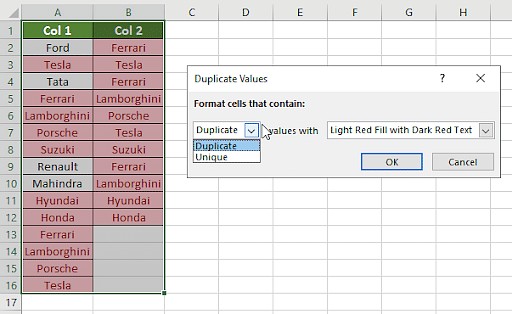
5. How do I compare two columns in Excel and highlight the duplicates?

To compare two columns in Excel and highlight the duplicates, follow these steps:

1. Select the two columns you want to compare.
2. Go to the Home tab and click on Conditional Formatting.
3. Choose “Highlight Cells Rules” and select “Duplicate Values” from the dropdown menu.
4. In the Duplicate Values dialog box, make sure “Duplicate” is selected.
5. Choose a formatting style or leave the default style.
6. Click OK.

6. Is it possible to compare two columns in Excel using the Index-Match function?

Yes, you can compare two columns in Excel using the Index-Match function. This combination is more flexible than VLOOKUP, especially when dealing with complex data structures.

7. How to compare multiple columns in Excel?

To compare multiple columns in Excel, you can use the conditional formatting option on the home and format the setting to “duplicates” or “uniques”, and choose the desired color to highlight the values to compare multiple columns.

8. How do you compare two lists in Excel for matches?

You can compare two lists in Excel using IF function, MATCH function or highlighting row differences.

9. How do I compare two columns in Excel and highlight the duplicates?

To compare two columns in Excel and highlight the duplicates, follow these steps:

1. Select the two columns you want to compare.
2. Go to the Home tab and click on Conditional Formatting.
3. Choose “Highlight Cells Rules” and select “Duplicate Values” from the dropdown menu.
4. In the Duplicate Values dialog box, make sure “Duplicate” is selected.
5. Choose a formatting style or leave the default style.
6. Click OK.

10. What are some common mistakes to avoid when comparing columns in Excel?

Some common mistakes to avoid when comparing columns in Excel include not cleaning data, using the wrong method, making errors in formulas, and not documenting steps.

Ready to make data-driven decisions with confidence? Visit COMPARE.EDU.VN today at compare.edu.vn and explore our comprehensive comparison tools. Our expert analysis and user reviews will empower you to choose the best solutions for your needs. Contact us at 333 Comparison Plaza, Choice City, CA 90210, United States, or reach out via Whatsapp at +1 (626) 555-9090.