How To Compare 2 Columns In Excel Using VLOOKUP

Comparing two columns in Excel using VLOOKUP is a powerful technique for identifying matches and differences within your data. At COMPARE.EDU.VN, we provide expert guidance and practical examples to help you master this essential Excel skill, enabling you to analyze your data more effectively. This comprehensive guide will delve into various scenarios, offering solutions and techniques to compare data efficiently. By the end, you’ll be proficient in using VLOOKUP for data comparison, extracting common values, and spotting discrepancies.

1. Understanding the Basics of VLOOKUP for Column Comparison

The VLOOKUP function is a cornerstone of data analysis in Excel, primarily used for looking up and retrieving data from a table based on a specific value. However, it can also be cleverly employed to compare two columns and identify matching or missing data. To effectively use VLOOKUP, it’s crucial to understand its syntax and how it operates. The basic syntax is as follows:

VLOOKUP(lookup_value, table_array, col_index_num, [range_lookup])

lookup_value: The value you want to search for in the first column of the table.
table_array: The range of cells that contains the table where you want to look for the value.
col_index_num: The column number in the table_array from which to return a matching value.
[range_lookup]: An optional argument that specifies whether you want to find an exact match (FALSE) or an approximate match (TRUE). For comparing columns, we almost always use FALSE to ensure accuracy.

When comparing two columns, you’ll typically use a value from one column as the lookup_value and the other column as the table_array. The function will then search for the lookup_value within the table_array and return a corresponding value.

For instance, consider two lists: one of customer IDs in column A and another of order IDs in column B. You want to find out which customer IDs have corresponding order IDs. Here’s how you can use VLOOKUP:

=VLOOKUP(A2, $B$2:$B$100, 1, FALSE)

In this formula:

A2 is the first customer ID you want to look up.
$B$2:$B$100 is the range containing the order IDs (List 2). The dollar signs make this an absolute reference, preventing it from changing when you copy the formula down.
1 indicates that you want to return the value from the first column of the table array (which is the order ID itself).
FALSE ensures you are looking for an exact match.

This formula will return the order ID if the customer ID is found in the order ID list. If the customer ID is not found, VLOOKUP will return a #N/A error, indicating a missing value.

2. Step-by-Step Guide: Comparing Two Columns for Common Values

Identifying common values between two columns is a frequent task in data analysis. VLOOKUP can efficiently accomplish this. Here’s a detailed guide:

Step 1: Set Up Your Data
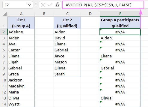
Assume you have two columns of data: Column A contains a list of names (List 1), and Column C contains another list of names (List 2). You want to find out which names from List 1 also appear in List 2.

Step 2: Write the VLOOKUP Formula
In a new column (e.g., Column E), enter the following formula in cell E2:

=VLOOKUP(A2, $C$2:$C$10, 1, FALSE)

A2 is the name from List 1 that you are looking for in List 2.
$C$2:$C$10 is the range of cells containing List 2.
1 indicates that you want to return the value from the first column of the table array (which is the name itself).
FALSE ensures an exact match.

Step 3: Apply the Formula to the Entire Column
Drag the fill handle (the small square at the bottom-right of cell E2) down to apply the formula to all the names in List 1. This will search for each name from List 1 in List 2.

Step 4: Interpret the Results

If a name from List 1 is found in List 2, the formula will return that name in Column E.
If a name is not found, the formula will return a #N/A error.

Step 5: Handle #N/A Errors (Optional)
To make the results cleaner, you can use the IFNA function to replace the #N/A errors with a more readable value, such as an empty string or a custom message. Modify the formula as follows:

=IFNA(VLOOKUP(A2, $C$2:$C$10, 1, FALSE), "")

This revised formula will return an empty string (“”) instead of #N/A, making it easier to see which names are not in List 2. You can also use a custom message like “Not Found” for clarity.

Step 6: Filter for Common Values (Optional)
If you want to create a list of only the common values, you can apply a filter to Column E. Select Column E, go to the “Data” tab, and click on “Filter.” Then, click the filter dropdown in cell E1 and uncheck the “(Blanks)” option (if you used the IFNA function) or the “#N/A” option. This will display only the names that are present in both lists.

By following these steps, you can efficiently identify and extract common values between two columns using VLOOKUP.

3. Finding Missing Values: Identifying Differences with VLOOKUP

Another common use case is to find values that exist in one column but not in another. This is crucial for identifying discrepancies and incomplete data. Here’s how to do it:

Step 1: Set Up Your Data
As before, assume you have two columns of data: Column A contains a list of names (List 1), and Column C contains another list of names (List 2). You want to find out which names from List 1 are missing from List 2.

Step 2: Write the Formula with ISNA and IF
In a new column (e.g., Column E), enter the following formula in cell E2:

=IF(ISNA(VLOOKUP(A2, $C$2:$C$10, 1, FALSE)), A2, "")

VLOOKUP(A2, $C$2:$C$10, 1, FALSE) searches for the name from List 1 in List 2.
ISNA() checks if the VLOOKUP result is #N/A (i.e., not found). If it is #N/A, ISNA returns TRUE; otherwise, it returns FALSE.
IF(ISNA(...), A2, "") checks the result of the ISNA function. If it’s TRUE (the name is not found), the formula returns the name from List 1 (A2); otherwise, it returns an empty string (“”).

Step 3: Apply the Formula to the Entire Column
Drag the fill handle down to apply the formula to all the names in List 1.

Step 4: Interpret the Results

If a name from List 1 is not found in List 2, the formula will return that name in Column E.
If a name is found, the formula will return an empty string.

Step 5: Filter for Missing Values (Optional)
To create a list of only the missing values, apply a filter to Column E. Select Column E, go to the “Data” tab, and click on “Filter.” Then, click the filter dropdown in cell E1 and uncheck the “(Blanks)” option. This will display only the names that are missing from List 2.

This approach allows you to quickly identify and list the values that are present in one column but not in the other, making it easier to manage and correct your data.

4. Comparing Columns in Different Sheets or Workbooks

Often, the data you need to compare resides in different sheets or even different workbooks. VLOOKUP can handle this scenario as well. Here’s how:

Step 1: Set Up Your Data
Assume you have List 1 in Column A on Sheet1 and List 2 in Column A on Sheet2. You want to find common values.

Step 2: Write the VLOOKUP Formula with Sheet References
In Sheet1, enter the following formula in cell B2:

=VLOOKUP(A2, Sheet2!$A$2:$A$10, 1, FALSE)

A2 is the name from List 1 in Sheet1 that you are looking for in List 2 on Sheet2.
Sheet2!$A$2:$A$10 is the range of cells containing List 2 on Sheet2.
1 indicates that you want to return the value from the first column of the table array (which is the name itself).
FALSE ensures an exact match.

Step 3: Apply the Formula to the Entire Column
Drag the fill handle down to apply the formula to all the names in List 1 on Sheet1.

Step 4: Interpret the Results
The results will be the same as when comparing columns on the same sheet. The formula will return the name if found in Sheet2 and a #N/A error if not found.

Step 5: Handle #N/A Errors (Optional)
Use the IFNA function to replace the #N/A errors with a more readable value:

=IFNA(VLOOKUP(A2, Sheet2!$A$2:$A$10, 1, FALSE), "")

Comparing Columns in Different Workbooks
The process is similar when comparing columns in different workbooks. The only difference is that the table_array reference will include the workbook name in square brackets. For example:

=VLOOKUP(A2, [Workbook2.xlsx]Sheet1!$A$2:$A$10, 1, FALSE)

Ensure that the other workbook is open when you use this formula. If the workbook is closed, the formula will return an error until the workbook is opened.

5. Advanced Techniques: Using FILTER with VLOOKUP

For Excel 365 users, the FILTER function can be combined with VLOOKUP to create more dynamic and efficient solutions. Here are a couple of examples:

Returning Common Values Dynamically
To return a list of common values without gaps, you can use the FILTER function in combination with the IFNA function and VLOOKUP:

=FILTER(A2:A10, IFNA(VLOOKUP(A2:A10, C2:C10, 1, FALSE), "")<>"")

A2:A10 is the range of cells containing List 1.
C2:C10 is the range of cells containing List 2.
VLOOKUP(A2:A10, C2:C10, 1, FALSE) searches for each value from List 1 in List 2.
IFNA(..., "") replaces the #N/A errors with empty strings.
FILTER(A2:A10, ...<>"") filters the values from List 1, keeping only those for which the VLOOKUP result is not an empty string (i.e., the values that are found in List 2).

This formula dynamically returns a list of common values without any gaps.

Returning Missing Values Dynamically
Similarly, to return a list of missing values dynamically, you can use the FILTER function with the ISNA function and VLOOKUP:

=FILTER(A2:A10, ISNA(VLOOKUP(A2:A10, C2:C10, 1, FALSE)))

A2:A10 is the range of cells containing List 1.
C2:C10 is the range of cells containing List 2.
VLOOKUP(A2:A10, C2:C10, 1, FALSE) searches for each value from List 1 in List 2.
ISNA(...) checks if the VLOOKUP result is #N/A (i.e., not found).
FILTER(A2:A10, ISNA(...)) filters the values from List 1, keeping only those for which the VLOOKUP result is #N/A (i.e., the values that are not found in List 2).

This formula dynamically returns a list of missing values without any gaps.

6. Alternative Functions: XLOOKUP and INDEX/MATCH

While VLOOKUP is a powerful tool, there are alternative functions that can also be used for comparing columns, each with its own advantages.

XLOOKUP
XLOOKUP is the modern successor to VLOOKUP and HLOOKUP, available in Excel 365 and Excel 2021. It offers several advantages over VLOOKUP, including:

No need to specify the column index number: XLOOKUP can return values from any column in the table, regardless of its position.
Handles errors internally: XLOOKUP has an optional if_not_found argument that allows you to specify a value to return if no match is found, eliminating the need for the IFNA function.
Supports approximate and exact matches: XLOOKUP can perform both approximate and exact matches, and it defaults to an exact match, making it less prone to errors.

Here’s how you can use XLOOKUP to compare two columns for common values:

=XLOOKUP(A2, C2:C10, C2:C10, "")

A2 is the value from List 1 that you are looking for in List 2.
C2:C10 is the range of cells containing List 2 (the lookup array).
C2:C10 is also the range of cells from which to return a value if a match is found (the return array).
"" is the value to return if no match is found.

To find missing values, you can use XLOOKUP with the FILTER function:

=FILTER(A2:A10, XLOOKUP(A2:A10, C2:C10, C2:C10, "")="")

This formula filters the values from List 1, keeping only those for which the XLOOKUP result is an empty string (i.e., the values that are not found in List 2).

INDEX/MATCH
The INDEX/MATCH combination is another powerful alternative to VLOOKUP. It is more flexible and less prone to errors than VLOOKUP because it does not rely on column numbers. Instead, it uses the MATCH function to find the position of a value in a list and then uses the INDEX function to return the value at that position from another list.

Here’s how you can use INDEX/MATCH to compare two columns for common values:

=IFNA(INDEX(C2:C10, MATCH(A2, C2:C10, 0)), "")

A2 is the value from List 1 that you are looking for in List 2.
C2:C10 is the range of cells containing List 2.
MATCH(A2, C2:C10, 0) finds the position of the value from List 1 in List 2. The 0 specifies an exact match.
INDEX(C2:C10, ...) returns the value from List 2 at the position found by the MATCH function.
IFNA(..., "") replaces the #N/A errors with empty strings.

To find missing values, you can use INDEX/MATCH with the IF and ISNA functions:

=IF(ISNA(MATCH(A2, C2:C10, 0)), A2, "")

This formula checks if the MATCH function returns #N/A (i.e., the value is not found). If it is, the formula returns the value from List 1; otherwise, it returns an empty string.

7. Identifying Matches and Differences with Text Labels

In some cases, you may want to add text labels to your data to indicate whether each value is present in both lists or only in one list. This can make your results more readable and easier to understand. Here’s how you can do it using VLOOKUP and other functions:

Using VLOOKUP with IF and ISNA
You can use the VLOOKUP formula together with the IF and ISNA functions to add text labels. For example:

=IF(ISNA(VLOOKUP(A2, $C$2:$C$10, 1, FALSE)), "Not in List 2", "In List 2")

A2 is the value from List 1 that you are looking for in List 2.
$C$2:$C$10 is the range of cells containing List 2.
VLOOKUP(A2, $C$2:$C$10, 1, FALSE) searches for the value from List 1 in List 2.
ISNA(...) checks if the VLOOKUP result is #N/A (i.e., not found).
IF(ISNA(...), "Not in List 2", "In List 2") checks the result of the ISNA function. If it’s TRUE (the value is not found), the formula returns “Not in List 2”; otherwise, it returns “In List 2”.

This formula will add a label to each value in List 1, indicating whether it is present in List 2 or not.

Using MATCH with IF and ISNA
You can also use the MATCH function with the IF and ISNA functions to achieve the same result:

=IF(ISNA(MATCH(A2, $C$2:$C$10, 0)), "Not in List 2", "In List 2")

A2 is the value from List 1 that you are looking for in List 2.
$C$2:$C$10 is the range of cells containing List 2.
MATCH(A2, $C$2:$C$10, 0) finds the position of the value from List 1 in List 2.
ISNA(...) checks if the MATCH function returns #N/A (i.e., not found).
IF(ISNA(...), "Not in List 2", "In List 2") checks the result of the ISNA function. If it’s TRUE (the value is not found), the formula returns “Not in List 2”; otherwise, it returns “In List 2”.

This formula provides the same labels as the VLOOKUP-based formula but uses the MATCH function instead.

8. Comparing Two Columns and Returning a Value from a Third Column

In some scenarios, you may need to compare two columns and, if a match is found, return a corresponding value from a third column. This is a common use case when working with tables containing related data. Here’s how you can do it using VLOOKUP, INDEX/MATCH, and XLOOKUP:

Using VLOOKUP
The VLOOKUP function is designed for this purpose. Suppose you have two tables: one with customer IDs and names (Table 1) and another with customer IDs and order dates (Table 2). You want to compare the customer IDs in both tables and, if a match is found, return the order date from Table 2.

Here’s the formula:

=VLOOKUP(A2, $D$2:$E$10, 2, FALSE)

A2 is the customer ID from Table 1 that you are looking for in Table 2.
$D$2:$E$10 is the range of cells containing Table 2 (customer IDs and order dates).
2 indicates that you want to return the value from the second column of Table 2 (the order date).
FALSE ensures an exact match.

This formula will return the order date if the customer ID is found in Table 2. If the customer ID is not found, the formula will return a #N/A error.

To handle #N/A errors, you can use the IFNA function:

=IFNA(VLOOKUP(A2, $D$2:$E$10, 2, FALSE), "")

This formula will return an empty string instead of #N/A, making the results cleaner.

Using INDEX/MATCH
The INDEX/MATCH combination provides a more flexible alternative to VLOOKUP. Here’s how you can use it to achieve the same result:

=IFNA(INDEX($E$2:$E$10, MATCH(A2, $D$2:$D$10, 0)), "")

A2 is the customer ID from Table 1 that you are looking for in Table 2.
$D$2:$D$10 is the range of cells containing the customer IDs in Table 2.
$E$2:$E$10 is the range of cells containing the order dates in Table 2.
MATCH(A2, $D$2:$D$10, 0) finds the position of the customer ID from Table 1 in the customer ID list in Table 2.
INDEX($E$2:$E$10, ...) returns the order date from Table 2 at the position found by the MATCH function.
IFNA(..., "") replaces the #N/A errors with empty strings.

This formula provides the same result as the VLOOKUP-based formula but uses the INDEX/MATCH combination instead.

Using XLOOKUP
XLOOKUP simplifies this task even further. Here’s the formula:

=XLOOKUP(A2, $D$2:$D$10, $E$2:$E$10, "")

A2 is the customer ID from Table 1 that you are looking for in Table 2.
$D$2:$D$10 is the range of cells containing the customer IDs in Table 2.
$E$2:$E$10 is the range of cells containing the order dates in Table 2.
"" is the value to return if no match is found.

XLOOKUP handles the error internally, making the formula more concise and easier to read.

9. Best Practices for Using VLOOKUP to Compare Columns

To ensure accurate and efficient data comparison, follow these best practices when using VLOOKUP:

Use Absolute References: Always use absolute references (e.g., $A$2:$A$10) for the table_array argument to prevent the range from changing when you copy the formula to other cells.
Ensure Exact Matches: Use FALSE for the range_lookup argument to ensure that you are looking for exact matches. This is crucial for accurate data comparison.
Handle Errors Gracefully: Use the IFNA function to replace #N/A errors with more readable values, such as empty strings or custom messages. This makes the results cleaner and easier to understand.
Sort Data: If you are using VLOOKUP for approximate matches (which is rare when comparing columns), make sure that the first column of the table_array is sorted in ascending order.
Consider Alternatives: Evaluate whether XLOOKUP or INDEX/MATCH might be more appropriate for your specific use case. These functions can be more flexible and less prone to errors than VLOOKUP.
Test Your Formulas: Always test your formulas with a small sample of data to ensure that they are working correctly before applying them to the entire dataset.
Document Your Formulas: Add comments to your formulas to explain what they are doing. This can be helpful for others who need to understand or modify your formulas in the future.

10. Common Issues and Troubleshooting

When using VLOOKUP to compare columns, you may encounter some common issues. Here are some troubleshooting tips:

#N/A Errors: This error indicates that the lookup_value was not found in the table_array. Check the following:
- Make sure that the lookup_value exists in the first column of the table_array.
- Ensure that you are using FALSE for the range_lookup argument to look for exact matches.
- Check for typos or inconsistencies in the data.
Incorrect Results: If your formula is returning incorrect results, check the following:
- Make sure that the col_index_num argument is correct. It should be the column number in the table_array from which you want to return a value.
- Ensure that you are using absolute references for the table_array argument.
- Check for data type mismatches. For example, if you are comparing numbers, make sure that both columns are formatted as numbers.
Performance Issues: If you are working with large datasets, VLOOKUP can be slow. Consider using XLOOKUP or INDEX/MATCH, which can be more efficient. Also, make sure that your data is properly indexed.
Formula Errors: If you are getting formula errors, check the syntax of your formula. Make sure that you have the correct number of arguments and that the arguments are in the correct order.

FAQ: Mastering VLOOKUP for Column Comparisons

1. What is the main advantage of using VLOOKUP to compare columns in Excel?

VLOOKUP allows you to quickly identify common or missing values between two lists, saving time and ensuring data accuracy.

2. How do I handle #N/A errors when using VLOOKUP for comparison?

Use the IFNA function to replace #N/A errors with custom text or blank cells for cleaner results.

3. Can I compare columns in different Excel sheets using VLOOKUP?

Yes, reference the other sheet in the table_array argument, like so: Sheet2!$A$2:$A$10.

4. What is the difference between VLOOKUP and XLOOKUP?

XLOOKUP is more flexible, doesn’t require specifying the column index number, handles errors internally, and defaults to exact matches.

5. How can I return a value from a third column based on the comparison of two columns?

Use VLOOKUP with the col_index_num argument set to the third column, or use INDEX/MATCH/XLOOKUP for more flexibility.

6. What does the FALSE argument in VLOOKUP do?

It ensures that VLOOKUP looks for an exact match, which is crucial for accurate column comparisons.

7. How do I use VLOOKUP to find missing values between two columns?

Combine VLOOKUP with the ISNA and IF functions to return values present in one column but not the other.

8. What are some alternatives to VLOOKUP for comparing columns?

XLOOKUP and INDEX/MATCH are excellent alternatives that offer more flexibility and efficiency.

9. Is it necessary to sort data when using VLOOKUP for column comparison?

No, sorting is not necessary when using FALSE for exact matches.

10. How can I dynamically filter common values using VLOOKUP?

Use the FILTER function in combination with VLOOKUP and IFNA to create a dynamic list of common values without gaps.

Conclusion: Leverage COMPARE.EDU.VN for Excel Mastery

Mastering the VLOOKUP function for comparing columns in Excel is a valuable skill that can greatly enhance your data analysis capabilities. Whether you need to find common values, identify missing data, or return values from related tables, VLOOKUP and its alternatives provide powerful tools for achieving your goals. By following the techniques and best practices outlined in this guide, you can efficiently and accurately compare your data and make informed decisions.

For further assistance and more detailed comparisons, be sure to visit COMPARE.EDU.VN. Our comprehensive resources and expert guidance can help you unlock the full potential of Excel and other data analysis tools. At COMPARE.EDU.VN, we are dedicated to providing you with the knowledge and skills you need to succeed in today’s data-driven world.

Ready to take your Excel skills to the next level? Visit compare.edu.vn today to explore more tutorials, tips, and resources. Contact us at 333 Comparison Plaza, Choice City, CA 90210, United States, or reach out via WhatsApp at +1 (626) 555-9090. Your journey to Excel mastery starts here