Comparing data in Excel is a common task, and highlighting matches between two columns is a quick way to identify similarities. This comprehensive guide provides various techniques to compare two Excel columns and highlight matching data, catering to different scenarios and desired outcomes.
Comparing Columns for Exact Row Matches
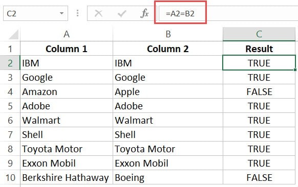
The simplest comparison involves a row-by-row check for identical data.
Using the Equals Sign
To determine if cells in the same row match, use the equals sign (=). For example, =A2=B2 returns TRUE if the values in A2 and B2 are identical, and FALSE otherwise. This formula can be copied down to compare entire columns.
Using the IF Function
For more descriptive results, use the IF function. =IF(A2=B2,"Match","Mismatch") returns “Match” for identical values and “Mismatch” for differences. For case-sensitive comparisons, use the EXACT function: =IF(EXACT(A2,B2),"Match","Mismatch"). This distinguishes between “apple” and “Apple”.
Highlighting Matching Rows with Conditional Formatting
To visually highlight matching rows, use Conditional Formatting:
- Select the data range.
- Go to Home > Conditional Formatting > New Rule.
- Choose Use a formula to determine which cells to format.
- Enter the formula
=$A1=$B1. The dollar sign ($) before the row number ensures the formula applies to the entire row. - Click Format and choose a highlighting style.
- Click OK.
Comparing Columns and Highlighting Matches Across Rows
This method highlights matches regardless of their row position, useful for finding duplicates within two columns.
Highlighting Duplicate Values
- Select the data range.
- Go to Home > Conditional Formatting > Highlight Cells Rules > Duplicate Values.
- Choose a formatting style and click OK. This highlights all duplicate values in both columns.
Highlighting Unique Values
To highlight values appearing in only one column, follow the same steps as above, but select Unique Values instead of Duplicate Values in the Conditional Formatting dialog box.
Finding Missing Data Points
To identify data points present in one column but missing in the other, use lookup functions.
Using VLOOKUP or MATCH
The formula =ISERROR(VLOOKUP(A2,$B$2:$B$10,1,0)) or =NOT(ISNUMBER(MATCH(A2,$B$2:$B$10,0))) returns TRUE if a value in column A is not found in column B. Filtering for TRUE reveals the missing data points. The MATCH function is generally preferred for its flexibility.
Comparing and Extracting Matching Data
To retrieve data from one column based on matches in another, use lookup functions.
Exact Match
=VLOOKUP(D2,$A$2:$B$14,2,0) or =INDEX($A$2:$B$14,MATCH(D2,$A$2:$A$14,0),2) returns the value from column B corresponding to a matching value in column D.
Partial Match
For approximate matches, use wildcard characters: =VLOOKUP("*"&D2&"*",$A$2:$B$14,2,0) or =INDEX($A$2:$B$14,MATCH("*"&D2&"*",$A$2:$A$14,0),2). This finds matches even with slight variations in text.
This guide provides a comprehensive overview of various methods to compare two columns in Excel and highlight matches. Choose the technique that best suits your specific needs and data structure. Remember to adjust formulas and ranges to match your actual data.