How to Compare 2 Columns for Duplicates in Excel

Comparing two columns for duplicates in Excel is a common task in data analysis, and COMPARE.EDU.VN can help you find the best method. This guide provides step-by-step instructions using various Excel features like conditional formatting, formulas, and functions to identify matching or unique entries. Discover effective techniques for duplicate identification, data comparison, and cell matching to streamline your data analysis process.

1. Understanding Column Comparison in Excel

Comparing columns in Excel involves checking corresponding cells across different columns to identify similarities or differences. This process is crucial for various tasks, including data validation, duplicate detection, and identifying discrepancies. It’s an essential skill for anyone working with spreadsheets and seeking to maintain data integrity.

2. Methods for Comparing Two Columns in Excel

Excel offers several methods to compare two columns for duplicates, each with its own strengths and weaknesses. Here are some of the most effective techniques:

2.1. Conditional Formatting

Conditional formatting is a quick and visual way to highlight duplicate or unique values in two columns. This method is useful for identifying patterns at a glance.

Steps:

1. Select the Range: Select both columns of data you want to compare.
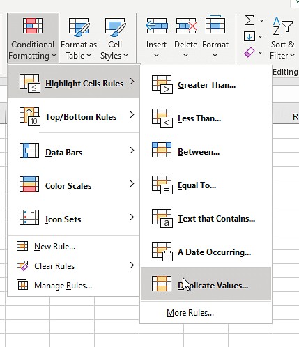
2. Access Conditional Formatting: Go to the “Home” tab and click on “Conditional Formatting” in the “Styles” group.
3. Highlight Duplicate Values: Choose “Highlight Cells Rules” and then “Duplicate Values.”
4. Choose Formatting: Select the formatting style you prefer (e.g., light red fill with dark red text) and click “OK.”

Excel will automatically highlight all duplicate values in the selected columns. You can also choose “Unique” in the “Duplicate Values” dialog box to highlight unique entries. This method is great for quickly visualizing matches but doesn’t provide a separate column indicating the comparison result. Using conditional formatting is a fast way to implement data highlighting, duplicate value identification, and conditional formatting rules.

2.2. Using the Equals Operator (=)

The equals operator is a simple formula-based approach to compare corresponding cells in two columns and return “TRUE” if they match or “FALSE” if they don’t.

Steps:

1. Create a New Column: Insert a new column next to the columns you want to compare.
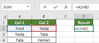
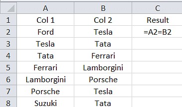
2. Enter the Formula: In the first cell of the new column (e.g., C2), enter the formula =A2=B2, where A2 and B2 are the first cells in the two columns you’re comparing.
3. Apply the Formula: Drag the fill handle (the small square at the bottom-right of the cell) down to apply the formula to all the rows.

Excel will display “TRUE” for rows where the values in the two columns match and “FALSE” where they don’t. You can further customize this by using an IF statement to display custom messages like “Match” or “No Match.” This technique is effective for direct cell comparison and creating an explicit comparison column. The equals operator offers direct comparison, formula-based approach, and cell matching.

2.3. The VLOOKUP Function

VLOOKUP (Vertical Lookup) is a powerful function to check if a value from one column exists in another column. It searches for a value in the first column of a range and returns a corresponding value from another column in the same row.

Formula:

=VLOOKUP(lookup_value, table_array, col_index_num, [range_lookup])

• lookup_value: The value you want to search for (e.g., the value in cell A2).
• table_array: The range where you want to search for the lookup value (e.g., $B$2:$B$10, using absolute references to prevent the range from changing when you drag the formula).
• col_index_num: The column number in the table_array from which to return a value. Since we’re just checking for existence, this can be any column in the table_array.
• [range_lookup]: An optional argument. Use FALSE for an exact match.

Steps:

1. Create a New Column: Insert a new column next to the columns you want to compare.
2. Enter the Formula: In the first cell of the new column (e.g., C2), enter the formula =IF(ISNA(VLOOKUP(A2,$B$2:$B$10,1,FALSE)),"Not Found","Found").
3. Apply the Formula: Drag the fill handle down to apply the formula to all the rows.

This formula checks if the value in cell A2 is found in the range B2:B10. If VLOOKUP returns an error (meaning the value is not found), the IFERROR function displays “Not Found.” Otherwise, it displays “Found.” This function is useful when you need to locate matching entries and identify missing values. VLOOKUP excels at finding matching entries, locating missing values, and enabling range lookup.

2.4. Using the IF Formula

The IF formula allows you to define a condition and return different values based on whether the condition is TRUE or FALSE. This is useful for customized comparisons.

Formula:

=IF(condition, value_if_true, value_if_false)

Steps:

1. Create a New Column: Insert a new column next to the columns you want to compare.
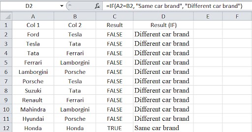
2. Enter the Formula: In the first cell of the new column (e.g., C2), enter the formula =IF(A2=B2,"Match","No Match").
3. Apply the Formula: Drag the fill handle down to apply the formula to all the rows.

This formula compares the values in cells A2 and B2. If they are equal, it displays “Match”; otherwise, it displays “No Match.” The IF formula is ideal for defining custom logic, returning custom messages, and enabling conditional logic.

2.5. The EXACT Formula

The EXACT formula compares two strings and returns TRUE only if they are exactly the same, including case sensitivity.

Formula:

=EXACT(text1, text2)

Steps:

1. Create a New Column: Insert a new column next to the columns you want to compare.
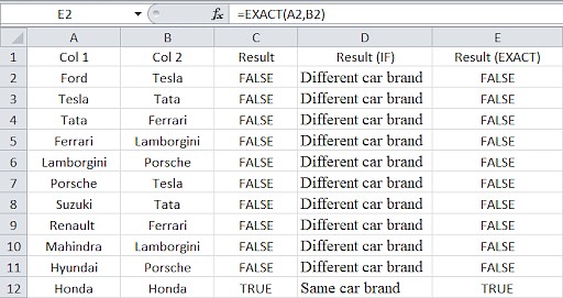
2. Enter the Formula: In the first cell of the new column (e.g., C2), enter the formula =EXACT(A2,B2).
3. Apply the Formula: Drag the fill handle down to apply the formula to all the rows.

Excel will display “TRUE” if the values in A2 and B2 are exactly the same (case-sensitive) and “FALSE” otherwise. The EXACT formula is useful when case sensitivity is crucial, comparing two strings, and performing exact comparison.

3. Choosing the Right Method for Your Scenario

The best method for comparing two columns in Excel depends on your specific needs and the type of data you’re working with. Here’s a summary to help you choose:

Method	Use Case	Advantages	Disadvantages
Conditional Formatting	Quickly visualizing duplicates or unique values.	Easy to use, visual, good for quick overviews.	Doesn’t provide a separate comparison column, limited customization.
Equals Operator (=)	Direct cell-by-cell comparison with a simple TRUE/FALSE result.	Simple formula, easy to understand, creates an explicit comparison column.	Limited customization, doesn’t handle complex matching criteria.
VLOOKUP Function	Checking if values from one column exist in another column.	Can find matches and identify missing values, flexible with IFERROR.	More complex formula, can be slower with large datasets.
IF Formula	Customized comparisons based on specific conditions.	Highly customizable, can return custom messages, supports conditional logic.	Requires more complex formula writing.
EXACT Formula	Case-sensitive comparisons.	Ensures exact matches, useful when case matters.	Case-sensitive, may not be suitable for all comparison scenarios.

4. Practical Scenarios and Examples

To further illustrate the use of these methods, let’s look at some practical scenarios:

4.1. Scenario 1: Comparing Two Columns Row-by-Row

Imagine you have two columns of customer IDs, and you want to check if the IDs match row by row.

Solution: Use the IF formula or the equals operator.

• IF Formula: =IF(A2=B2,"Match","No Match")
• Equals Operator: =A2=B2

If you need a case-sensitive comparison, use the EXACT formula:

• EXACT Formula: =IF(EXACT(A2, B2), "Match", " ")

4.2. Scenario 2: Comparing Multiple Columns for Row Matches

Suppose you have three columns (A, B, and C) and want to find rows where all three values match.

Solution: Use the AND function with the IF formula.

• Formula: =IF(AND(A2=B2, A2=C2), "Complete Match", " ")

This formula checks if the value in A2 is equal to both B2 and C2. If all conditions are true, it returns “Complete Match.” If you’re comparing a large number of columns, you can use the COUNTIF function for a more concise formula.

• Formula: =IF(COUNTIF($A2:$E2, $A2)=4, "Complete match," ")

In this case, we compare any two or more cells with the same values in the same row. The formula is as follows:

• Formula: =IF(OR(A2=B2, B2=C2, A2=C2), "Match", "")
• Formula: =IF(COUNTIF(B2:D2,A2)+COUNTIF(C2:D2,B2)+(C2=D2)=0,"Unique","Match")

4.3. Scenario 3: Compare Two Columns for Matches and Differences

You have two lists of product SKUs, and you want to find the SKUs that are present in list A but not in list B.

Solution: Use the COUNTIF function.

• Formula: =IF(COUNTIF($B:$B, $A2)=0, "Not Present in B", "")

This formula counts how many times the value in A2 appears in column B. If the count is 0, it means the value is not present in column B.

You can also use a single formula to get the result for matches and unique values:

• Formula: =IF(COUNTIF($B:$B, $A2)=0, "No Present in B", "Present in B")

4.4. Scenario 4: Compare Two Lists and Pull Matching Data

You have two lists: one with product IDs and names, and another with product IDs and prices. You want to create a new list that includes the product name and price for each matching product ID.

Solution: Use the VLOOKUP or INDEX MATCH formula.

• VLOOKUP Formula: =VLOOKUP(D2, $A$2:$B$6, 2, FALSE)
• INDEX MATCH Formula: =INDEX($B$2:$B$6, MATCH($D2, $A$2:$A$6, 0))
• XLOOKUP Formula: =XLOOKUP(D2, $A$2:$A$6, $B$2:$B$6)

These formulas search for the product ID in the second list (column D) within the first list (columns A and B) and return the corresponding product name or price.

4.5. Scenario 5: Highlight Row Matches and Differences

You want to highlight rows where all values in multiple columns are identical.

Solution: Use conditional formatting with a formula.

1. Select the Range: Select the columns you want to compare.
2. Access Conditional Formatting: Go to the “Home” tab and click on “Conditional Formatting.”
3. New Rule: Choose “New Rule…” and select “Use a formula to determine which cells to format.”
4. Enter the Formula: Enter the formula =AND($A2=$B2, $A2=$C2) or =COUNTIF($A2:$C2, $A2)=3.
5. Format: Click “Format…” and choose the formatting style you want to apply.
6. Click OK: Click “OK” to apply the conditional formatting.

This will highlight the rows where the values in columns A, B, and C are identical.

You can also find and highlight the matches and differences in Excel by following the steps below:

1. Select the Columns: Select the columns with the dataset you want to compare.
2. Go to “Find and Select”: Go to the editing group section on the Home tab, click the “Find and Select” drop-down, and choose “Go To Special.”
3. Select Row Differences: Select “Row Differences” and click OK.
4. Highlight Differences: The cells having different values than the cells compared in each row will be colored. To change the color, click the Fill Color icon and choose the color of your choice.

5. Advanced Tips and Tricks

Here are some additional tips and tricks to enhance your column comparison skills in Excel:

• Wildcards with VLOOKUP: Use wildcards like "*" to find partial matches. For example, if you want to find “Ford” in a column that contains “Ford India,” use VLOOKUP("Ford*",$B$2:$B$10,1,FALSE).
• Combining Formulas: Combine multiple formulas to handle complex scenarios. For example, use IF(AND(A2=B2, C2>D2), "Match", "No Match") to compare two columns and check if a value in another column is greater than another.
• Using Helper Columns: Create helper columns to break down complex comparisons into smaller, manageable steps.
• Filtering: Use Excel’s filtering capabilities to quickly display only the rows that match or don’t match your criteria.
• Data Validation: Implement data validation rules to prevent duplicates from being entered in the first place.

6. How COMPARE.EDU.VN Can Help

Comparing data in Excel can be time-consuming and complex. COMPARE.EDU.VN simplifies the process by providing comprehensive guides and tools to help you make informed decisions. Whether you’re comparing product features, service offerings, or any other data, COMPARE.EDU.VN offers detailed comparisons, user reviews, and expert insights to streamline your analysis.

Visit COMPARE.EDU.VN to discover more comparison tools and resources that can help you make smarter choices. Our platform offers a wide range of comparisons across various categories, ensuring you have the information you need to make the best decision for your specific needs. Contact us at 333 Comparison Plaza, Choice City, CA 90210, United States, or via Whatsapp at +1 (626) 555-9090 for personalized assistance.

7. FAQs

1. How to compare two columns in Excel?

One popular method for comparing two columns in Excel is to follow these steps: select both columns of data → go to the Home tab → click on Find & Select → choose Go To Special → select Row Differences → click OK.

2. Is it possible to compare two columns in Excel using the Index-Match function?

Yes, you can compare two columns in Excel using the Index-Match function by creating the required formula for the data required.

3. How to compare multiple columns in Excel?

To compare multiple columns in Excel, you can use the conditional formatting option on the home and format the setting to “duplicates” or “uniques”, and choose the desired color to highlight the values to compare multiple columns.

4. How do you compare two lists in Excel for matches?

You can compare two lists in Excel using IF function, MATCH function or highlighting row differences.

5. How do I compare two columns in Excel and highlight the duplicates?

To compare two columns in Excel and highlight the duplicates, follow these steps:

1. Select the two columns you want to compare.
2. Go to the Home tab and click on Conditional Formatting.
3. Choose “Highlight Cells Rules” and select “Duplicate Values” from the dropdown menu.
4. In the Duplicate Values dialog box, make sure “Duplicate” is selected.
5. Choose a formatting style or leave the default style.
6. Click OK.

Excel will then highlight the duplicate values in the selected columns, making them easy to identify.

6. Can I perform a case-sensitive comparison in Excel?

Yes, you can use the EXACT formula for case-sensitive comparisons. It returns TRUE only if the strings are exactly the same, including case.

7. How can I compare two columns and return a custom message based on the comparison?

Use the IF formula to define a condition and return different values based on whether the condition is TRUE or FALSE. For example, =IF(A2=B2,"Match","No Match").

8. What is the best method for comparing large datasets in Excel?

For large datasets, consider using VLOOKUP or INDEX MATCH formulas, but be aware of performance limitations. Ensure your formulas are optimized and consider using helper columns to break down complex comparisons.

9. How do I find the values that are present in one column but not in another?

Use the COUNTIF function to check if a value from the first column exists in the second column. For example, =IF(COUNTIF($B:$B, $A2)=0, "Not Present in B", "").

10. Can I use conditional formatting to highlight differences between two columns?

Yes, you can use conditional formatting with a formula to highlight differences. Select the columns, create a new rule, use a formula like =A2<>B2, and choose a formatting style to highlight the differences.

8. Conclusion

Comparing two columns for duplicates in Excel is a fundamental skill for data analysis. By mastering the techniques described in this guide, you can efficiently identify matches and differences, validate data, and streamline your spreadsheet workflows. Whether you’re using conditional formatting for a quick overview or complex formulas for detailed analysis, Excel provides the tools you need to get the job done.

For more detailed comparisons and expert insights, visit COMPARE.EDU.VN, your go-to source for making informed decisions. Contact us at 333 Comparison Plaza, Choice City, CA 90210, United States, or via Whatsapp at +1 (626) 555-9090. Start comparing today and make smarter choices with compare.edu.vn!