How to Compare 2 Cells in Excel and Highlight Differences

Comparing data in Excel is a common task, and understanding How To Compare 2 Cells In Excel And Highlight Differences is a valuable skill. At COMPARE.EDU.VN, we provide a comprehensive guide on cell comparison techniques, helping you identify matches and differences efficiently and effectively. Learn methods to analyze data effortlessly with advanced Excel features and highlighting techniques for quick data analysis.

1. Introduction: Mastering Cell Comparison in Excel with COMPARE.EDU.VN

Do you need to compare data in Excel but find it a daunting task? Identifying differences and similarities between cells can be crucial for data analysis and decision-making. Whether you’re a student, a professional, or just someone trying to manage data, COMPARE.EDU.VN offers the knowledge and tools you need to streamline your Excel comparisons. We’ll guide you through various methods, from simple formulas to advanced conditional formatting, ensuring you can master cell comparison and make informed decisions. By understanding these techniques, you can significantly improve your data handling skills. Learn effective cell comparison strategies, data matching in Excel, and highlighting techniques with COMPARE.EDU.VN’s detailed guidance.

2. Understanding the Basics of Cell Comparison

Before diving into advanced techniques, it’s essential to grasp the basics of comparing cells in Excel. This involves understanding how to use simple formulas to determine if two cells contain the same or different values.

2.1. Using the IF Function for Basic Comparison

The IF function is a fundamental tool for cell comparison. It allows you to check if a condition is true or false and return a specific value based on the result.

2.1.1. Formula for Matches

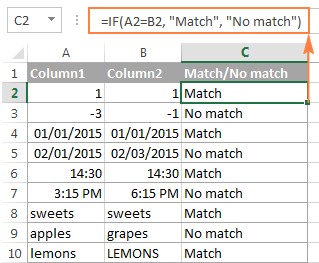
To find cells with identical content, you can use the following formula:

=IF(A1=B1,"Match","")

This formula compares the values in cells A1 and B1. If they are the same, it returns “Match”; otherwise, it returns an empty string.

2.1.2. Formula for Differences

To find cells with different values, simply replace the equals sign with the non-equality sign (<>):

=IF(A1<>B1,"No match","")

This formula returns “No match” if the values in A1 and B1 are different.

2.1.3. Combining Matches and Differences

You can combine both checks in a single formula:

=IF(A1=B1,"Match","No match")

Or:

=IF(A1<>B1,"No match","Match")

2.2. Handling Different Data Types

The IF function works well with various data types, including numbers, dates, times, and text strings. However, when comparing text, it’s important to consider case sensitivity.

2.2.1. Case-Insensitive Comparison

By default, Excel ignores case when comparing text values. For example, “Apple” and “apple” are considered the same.

2.2.2. Case-Sensitive Comparison with EXACT Function

To perform a case-sensitive comparison, use the EXACT function:

=IF(EXACT(A1,B1),"Match","No match")

The EXACT function returns TRUE if the cells are identical, including case, and FALSE otherwise.

3. Advanced Techniques for Cell Comparison

Beyond the basics, Excel offers advanced techniques to compare cells based on specific criteria and highlight the differences.

3.1. Conditional Formatting for Visual Comparison

Conditional formatting allows you to apply formatting to cells based on certain conditions. This is particularly useful for visually identifying matches and differences.

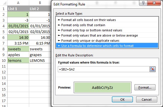
3.1.1. Highlighting Matches

To highlight cells with identical entries:

1. Select the cells you want to format.
2. Go to Conditional Formatting > New Rule > Use a formula to determine which cells to format.
3. Enter the formula: =$A1=$B1 (assuming row 1 is the first data row).
4. Choose a formatting style (e.g., fill color).

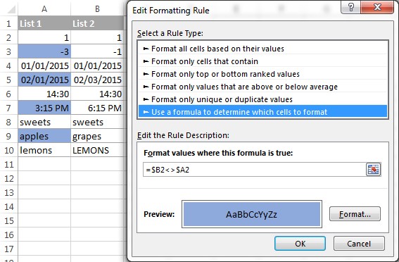
3.1.2. Highlighting Differences

To highlight cells with different entries, use the formula:

=$A1<>$B1

3.2. Using Named Ranges for Dynamic Comparison

Named ranges make your formulas more readable and easier to maintain. You can define a named range for each cell and use these names in your comparison formulas.

3.2.1. Defining Named Ranges

1. Select a cell (e.g., A1).
2. Go to the Formulas tab and click Define Name.
3. Enter a name (e.g., CellA1) and click OK.

3.2.2. Using Named Ranges in Formulas

You can now use the named ranges in your formulas:

=IF(CellA1=CellB1,"Match","No match")

3.3. Combining Functions for Complex Comparisons

You can combine multiple functions to perform more complex comparisons. For example, you can use the AND function to check multiple conditions.

3.3.1. Using AND Function

=IF(AND(A1>10,B1<20),"Condition Met","")

This formula checks if the value in A1 is greater than 10 AND the value in B1 is less than 20.

3.3.2. Using OR Function

=IF(OR(A1="Yes",B1="No"),"Condition Met","")

This formula checks if the value in A1 is “Yes” OR the value in B1 is “No”.

4. Comparing Multiple Cells

Sometimes, you need to compare more than two cells. Excel provides functions and techniques to handle multiple cell comparisons effectively.

4.1. Comparing Multiple Cells in the Same Row

You can use the AND or OR functions to compare multiple cells in the same row.

4.1.1. Finding Matches in All Cells

To find rows where all cells have the same value:

=IF(AND(A1=B1,A1=C1),"Full Match","")

4.1.2. Finding Matches in Any Two Cells

To find rows where any two cells have the same value:

=IF(OR(A1=B1,B1=C1,A1=C1),"Match","")

4.2. Using COUNTIF for Multiple Cell Comparison

The COUNTIF function can be used to count how many cells meet a certain criteria. This is useful for comparing multiple cells.

4.2.1. Counting Matches

=IF(COUNTIF(A1:C1,A1)=3,"Full Match","")

This formula checks if all three cells (A1, B1, and C1) have the same value.

5. Practical Examples of Cell Comparison

To illustrate the concepts, let’s look at some practical examples of cell comparison in Excel.

5.1. Comparing Product Prices

Suppose you have a list of product prices from two different suppliers and you want to identify any price discrepancies.

5.1.1. Data Setup

Product	Supplier A Price	Supplier B Price
Product 1	$10	$10
Product 2	$15	$12
Product 3	$20	$20
Product 4	$25	$22

5.1.2. Comparison Formula

In column D, enter the formula:

=IF(B2=C2,"Match","Price Difference")

This will show “Match” if the prices are the same and “Price Difference” if they are different.

5.1.3. Conditional Formatting

You can also use conditional formatting to highlight the price differences:

1. Select column D.
2. Go to Conditional Formatting > New Rule > Use a formula to determine which cells to format.
3. Enter the formula: =$B2<>$C2.
4. Choose a highlight color.

5.2. Comparing Dates

You can compare dates to check for deadlines, anniversaries, or other important events.

5.2.1. Data Setup

Task	Start Date	End Date
Task 1	1/1/2024	1/15/2024
Task 2	1/5/2024	1/20/2024
Task 3	1/10/2024	1/25/2024

5.2.2. Comparison Formula

In column D, enter the formula:

=IF(C2>TODAY(),"Upcoming","Overdue")

This will show “Upcoming” if the end date is in the future and “Overdue” if it is in the past.

5.2.3. Conditional Formatting

You can use conditional formatting to highlight overdue tasks:

1. Select column D.
2. Go to Conditional Formatting > New Rule > Use a formula to determine which cells to format.
3. Enter the formula: =$C2<TODAY().
4. Choose a highlight color.

5.3. Comparing Text Strings

You can compare text strings to check for consistency, spelling errors, or other discrepancies.

5.3.1. Data Setup

Item	Description A	Description B
Item 1	Apple	Apple
Item 2	Banana	Bannana
Item 3	Orange	Orange

5.3.2. Comparison Formula

In column D, enter the formula:

=IF(A2=B2,"Match","Spelling Error")

This will show “Match” if the text strings are the same and “Spelling Error” if they are different.

5.3.3. Conditional Formatting

You can use conditional formatting to highlight spelling errors:

1. Select column D.
2. Go to Conditional Formatting > New Rule > Use a formula to determine which cells to format.
3. Enter the formula: =$B2<>$C2.
4. Choose a highlight color.

6. Troubleshooting Common Issues

While comparing cells in Excel, you may encounter some common issues. Here’s how to troubleshoot them.

6.1. Incorrect Results

If you’re getting incorrect results, double-check your formulas. Make sure you’re using the correct cell references and comparison operators.

6.1.1. Checking Cell References

Ensure that your cell references are accurate. Use absolute references ($A$1) if you want the cell reference to remain constant when you copy the formula.

6.1.2. Verifying Comparison Operators

Make sure you’re using the correct comparison operators (=, <>, >, <, >=, <=).

6.2. Formulas Not Updating

Sometimes, formulas may not update automatically.

6.2.1. Recalculating the Worksheet

Press F9 to recalculate the entire worksheet.

6.2.2. Setting Calculation Options

Go to Formulas > Calculation Options and make sure it’s set to Automatic.

6.3. Conditional Formatting Not Working

If your conditional formatting isn’t working, check the following:

6.3.1. Formula Accuracy

Ensure that your conditional formatting formula is accurate.

6.3.2. Rule Priority

Check the rule priority in the Conditional Formatting Rules Manager. Rules are applied in order, so make sure the correct rule is at the top.

7. Using Excel Add-Ins for Advanced Comparison

For more advanced comparison tasks, consider using Excel add-ins. These add-ins offer additional features and capabilities that can streamline your workflow.

7.1. Ablebits Ultimate Suite

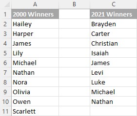
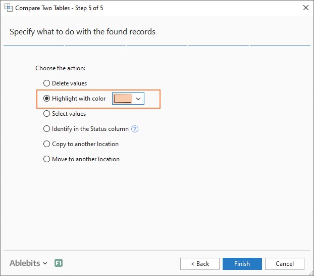
Ablebits Ultimate Suite includes a Compare Two Tables tool that allows you to compare two lists or tables based on multiple columns. It can identify matches and differences and highlight them.

7.1.1. Comparing Two Lists

1. Click the Compare Tables button on the Ablebits Data tab.
2. Select the first list and click Next.
3. Select the second list and click Next.
4. Choose whether to search for matches or differences.
5. Select the columns for comparison.
6. Choose how to deal with the found items (e.g., highlight with color or identify in a status column).

7.1.2. Highlighting Duplicates

You can highlight duplicates in the selected color:

7.2. Kutools for Excel

Kutools for Excel offers a variety of tools for data analysis, including comparison tools. It can help you compare ranges, sheets, and workbooks.

7.2.1. Comparing Ranges

1. Select the ranges you want to compare.
2. Go to the Kutools tab and choose the comparison tool.
3. Specify the comparison criteria and options.

8. Best Practices for Cell Comparison

To ensure accurate and efficient cell comparison, follow these best practices.

8.1. Keep Data Consistent

Ensure that your data is consistent and accurate. This includes checking for spelling errors, formatting inconsistencies, and other data quality issues.

8.2. Use Clear and Concise Formulas

Use clear and concise formulas that are easy to understand and maintain. Avoid overly complex formulas that can be difficult to troubleshoot.

8.3. Document Your Formulas

Document your formulas using comments. This will help you and others understand the purpose of the formula and how it works.

8.4. Test Your Formulas

Test your formulas thoroughly to ensure they’re producing accurate results. Use a variety of test cases to cover different scenarios.

8.5. Use Named Ranges

Use named ranges to make your formulas more readable and easier to maintain.

8.6. Apply Conditional Formatting Wisely

Apply conditional formatting wisely to highlight important information and make your data easier to understand.

9. Advanced Excel Functions for Cell Comparison

To enhance your cell comparison skills, explore these advanced Excel functions:

9.1. VLOOKUP

VLOOKUP is a powerful function for finding data in a table or range.

9.1.1. Syntax

=VLOOKUP(lookup_value, table_array, col_index_num, [range_lookup])

• lookup_value: The value to search for.
• table_array: The range of cells to search in.
• col_index_num: The column number in the table array to return the matching value from.
• range_lookup: An optional argument that specifies whether to find an exact or approximate match (TRUE for approximate, FALSE for exact).

9.1.2. Example

=VLOOKUP(A2,$E$2:$F$10,2,FALSE)

This formula searches for the value in A2 in the range E2:F10 and returns the value from the second column (column F) if an exact match is found.

9.2. INDEX MATCH

INDEX MATCH is a flexible alternative to VLOOKUP. It can perform more complex lookups and is less prone to errors.

9.2.1. Syntax

=INDEX(array, MATCH(lookup_value, lookup_array, [match_type]))

• array: The range of cells to return a value from.
• lookup_value: The value to search for.
• lookup_array: The range of cells to search in.
• match_type: An optional argument that specifies the type of match (0 for exact match).

9.2.2. Example

=INDEX($B$2:$B$10,MATCH(A2,$A$2:$A$10,0))

This formula searches for the value in A2 in the range A2:A10 and returns the corresponding value from the range B2:B10 if an exact match is found.

9.3. XLOOKUP

XLOOKUP is a modern lookup function that combines the capabilities of VLOOKUP and INDEX MATCH. It is available in Excel 365 and later versions.

9.3.1. Syntax

=XLOOKUP(lookup_value, lookup_array, return_array, [if_not_found], [match_mode], [search_mode])

• lookup_value: The value to search for.
• lookup_array: The range of cells to search in.
• return_array: The range of cells to return a value from.
• if_not_found: An optional argument that specifies the value to return if no match is found.
• match_mode: An optional argument that specifies the type of match (0 for exact match).
• search_mode: An optional argument that specifies the search direction.

9.3.2. Example

=XLOOKUP(A2,$A$2:$A$10,$B$2:$B$10,"Not Found",0)

This formula searches for the value in A2 in the range A2:A10 and returns the corresponding value from the range B2:B10 if an exact match is found. If no match is found, it returns “Not Found”.

10. Using AI for Enhanced Cell Comparison

Leveraging AI tools can significantly improve the speed and accuracy of cell comparison.

10.1. AI-Powered Excel Add-Ins

Several AI-powered Excel add-ins can assist with data analysis and comparison. These tools use machine learning algorithms to identify patterns, anomalies, and relationships in your data.

10.1.1. Microsoft Excel Insights

Microsoft Excel Insights uses AI to analyze your data and provide insights, such as trends, outliers, and correlations.

10.1.2. Third-Party AI Add-Ins

Explore third-party AI add-ins for Excel that offer advanced data analysis and comparison capabilities. These tools can automate repetitive tasks and provide deeper insights into your data.

10.2. Natural Language Processing (NLP)

NLP can be used to compare text strings and identify similarities and differences. This is particularly useful for analyzing large volumes of unstructured text data.

10.2.1. Text Comparison Tools

Use NLP-based text comparison tools to analyze text strings and identify semantic similarities and differences. These tools can provide a more nuanced understanding of your data than simple string matching.

11. Optimizing Excel Performance for Large Datasets

When working with large datasets, optimizing Excel performance is crucial.

11.1. Using Efficient Formulas

Use efficient formulas that minimize calculation time. Avoid volatile functions, such as NOW() and RAND(), which recalculate every time the worksheet changes.

11.2. Disabling Automatic Calculations

Disable automatic calculations and manually recalculate the worksheet when needed. Go to Formulas > Calculation Options and set it to Manual.

11.3. Using Arrays and Named Ranges

Use arrays and named ranges to reduce the number of calculations. Arrays can perform multiple calculations in a single formula, while named ranges can improve formula readability and maintainability.

11.4. Reducing Conditional Formatting

Reduce the use of conditional formatting, as it can slow down Excel. Use conditional formatting only when necessary and optimize the rules to minimize calculation time.

11.5. Using Excel Tables

Use Excel tables to manage your data. Tables offer several performance benefits, such as structured references and automatic expansion when you add new data.

12. Advanced Conditional Formatting Techniques

Explore these advanced conditional formatting techniques to further enhance your cell comparison skills:

12.1. Using Multiple Conditions

Use multiple conditions to apply different formatting based on different criteria.

12.1.1. Creating Multiple Rules

Create multiple conditional formatting rules for the same cells, each with different criteria and formatting styles.

12.1.2. Using AND and OR Functions

Use the AND and OR functions in your conditional formatting formulas to combine multiple conditions.

12.2. Using Icon Sets and Data Bars

Use icon sets and data bars to visually represent your data and highlight important values.

12.2.1. Applying Icon Sets

Apply icon sets to your cells to display icons based on the cell values.

12.2.2. Applying Data Bars

Apply data bars to your cells to display bars that represent the cell values relative to other values in the range.

12.3. Using Color Scales

Use color scales to apply a gradient of colors to your cells based on the cell values.

12.3.1. Applying Two-Color Scales

Apply a two-color scale to your cells to display a gradient of colors between two values.

12.3.2. Applying Three-Color Scales

Apply a three-color scale to your cells to display a gradient of colors between three values.

13. Advanced Data Validation Techniques

Data validation is a powerful tool for ensuring data accuracy and consistency.

13.1. Creating Custom Validation Rules

Create custom validation rules to restrict the values that can be entered into a cell.

13.1.1. Using Formulas

Use formulas in your data validation rules to create complex validation criteria.

13.1.2. Using Lists

Use lists in your data validation rules to restrict the values to a predefined set of options.

13.2. Displaying Error Messages

Display custom error messages to provide users with clear and helpful feedback when they enter invalid data.

13.2.1. Customizing Error Alerts

Customize the error alert messages to provide specific instructions and guidance to users.

13.2.2. Using Input Messages

Use input messages to provide users with instructions and guidance before they enter data.

14. Automating Cell Comparison with VBA

Automating cell comparison with VBA (Visual Basic for Applications) can save you time and effort.

14.1. Writing VBA Macros

Write VBA macros to automate repetitive cell comparison tasks.

14.1.1. Recording Macros

Record macros to capture your actions and generate VBA code.

14.1.2. Editing Macros

Edit your macros to customize them and add more complex logic.

14.2. Using VBA Functions

Use VBA functions to perform custom cell comparison tasks.

14.2.1. Creating Custom Functions

Create custom VBA functions to perform specific cell comparison tasks.

14.2.2. Calling Functions from Worksheets

Call your custom VBA functions from your worksheets to perform cell comparison tasks.

15. Data Cleaning and Preparation for Accurate Comparison

Accurate cell comparison relies on clean and well-prepared data.

15.1. Removing Duplicates

Remove duplicate rows and columns to ensure accurate comparison.

15.1.1. Using the Remove Duplicates Feature

Use the Remove Duplicates feature in Excel to quickly remove duplicate rows.

15.1.2. Using Formulas

Use formulas to identify and remove duplicate rows and columns.

15.2. Standardizing Data Formats

Standardize data formats to ensure consistent comparison.

15.2.1. Using the Format Cells Dialog

Use the Format Cells dialog to standardize data formats, such as dates, numbers, and text.

15.2.2. Using Formulas

Use formulas to convert data to a consistent format.

15.3. Handling Missing Data

Handle missing data to avoid errors and ensure accurate comparison.

15.3.1. Using the IF Function

Use the IF function to handle missing data and replace it with a default value.

15.3.2. Using the ISBLANK Function

Use the ISBLANK function to check for empty cells and handle them accordingly.

16. Comparing Data Across Multiple Worksheets and Workbooks

Comparing data across multiple worksheets and workbooks can be challenging, but Excel provides several tools to help.

16.1. Using 3D References

Use 3D references to refer to cells in multiple worksheets.

16.1.1. Creating 3D References

Create 3D references by specifying a range of worksheet names followed by a cell reference.

16.1.2. Using the INDIRECT Function

Use the INDIRECT function to create dynamic 3D references.

16.2. Using the Consolidate Feature

Use the Consolidate feature to combine data from multiple worksheets into a single worksheet.

16.2.1. Consolidating Data by Position

Consolidate data by position to combine data from the same cell locations in multiple worksheets.

16.2.2. Consolidating Data by Category

Consolidate data by category to combine data based on row and column labels.

16.3. Using Power Query

Use Power Query to import and transform data from multiple workbooks.

16.3.1. Importing Data from Multiple Workbooks

Import data from multiple workbooks into a single Power Query query.

16.3.2. Transforming and Combining Data

Transform and combine the data in Power Query to prepare it for comparison.

17. Using Pivot Tables for Advanced Data Comparison

Pivot tables are powerful tools for summarizing and analyzing data.

17.1. Creating Pivot Tables

Create pivot tables to summarize and analyze your data.

17.1.1. Selecting Data

Select the data you want to include in your pivot table.

17.1.2. Dragging Fields

Drag fields to the Rows, Columns, Values, and Filters areas to create your pivot table.

17.2. Using Calculated Fields

Use calculated fields to perform custom calculations in your pivot table.

17.2.1. Creating Calculated Fields

Create calculated fields to perform custom calculations based on the data in your pivot table.

17.2.2. Using Formulas

Use formulas in your calculated fields to perform more complex calculations.

17.3. Using Slicers and Filters

Use slicers and filters to filter your data and focus on specific subsets.

17.3.1. Adding Slicers

Add slicers to your pivot table to quickly filter the data.

17.3.2. Adding Filters

Add filters to your pivot table to filter the data based on specific criteria.

18. Exploring Excel Alternatives for Data Comparison

While Excel is a powerful tool, several alternatives offer specialized features for data comparison.

18.1. Google Sheets

Google Sheets is a web-based spreadsheet application that offers similar features to Excel.

18.1.1. Using Conditional Formatting

Use conditional formatting in Google Sheets to highlight matches and differences.

18.1.2. Using Formulas

Use formulas in Google Sheets to compare cells and perform calculations.

18.2. Apache OpenOffice Calc

Apache OpenOffice Calc is a free and open-source spreadsheet application.

18.2.1. Using Conditional Formatting

Use conditional formatting in Apache OpenOffice Calc to highlight matches and differences.

18.2.2. Using Formulas

Use formulas in Apache OpenOffice Calc to compare cells and perform calculations.

18.3. Dedicated Data Comparison Tools

Several dedicated data comparison tools offer advanced features for comparing and merging data.

18.3.1. WinMerge

WinMerge is a free and open-source differencing and merging tool for Windows.

18.3.2. Araxis Merge

Araxis Merge is a professional differencing and merging tool for Windows and macOS.

19. Compliance and Data Integrity in Cell Comparison

Maintaining compliance and data integrity is crucial in cell comparison.

19.1. Auditing and Tracking Changes

Implement auditing and tracking mechanisms to monitor changes to your data.

19.1.1. Using the Track Changes Feature

Use the Track Changes feature in Excel to track changes to your data.

19.1.2. Using VBA Macros

Use VBA macros to log changes to your data in a separate audit log.

19.2. Implementing Data Validation Rules

Implement data validation rules to prevent invalid data from being entered.

19.2.1. Creating Validation Rules

Create data validation rules to restrict the values that can be entered into a cell.

19.2.2. Customizing Error Messages

Customize error messages to provide users with clear and helpful feedback when they enter invalid data.

19.3. Ensuring Data Security

Ensure the security of your data by implementing appropriate access controls and encryption.

19.3.1. Using Password Protection

Use password protection to restrict access to your Excel files.

19.3.2. Using Encryption

Use encryption to protect your data from unauthorized access.

20. Conclusion: Achieving Data Clarity with COMPARE.EDU.VN

Mastering the art of how to compare 2 cells in Excel and highlight differences is more than just a technical skill; it’s a gateway to better data management and informed decision-making. With the techniques and strategies discussed in this comprehensive guide, you’re now equipped to tackle any cell comparison task with confidence. Whether you’re analyzing financial data, managing inventory, or tracking project progress, these skills will empower you to make data-driven decisions that drive success. Explore advanced comparison techniques, learn the benefits of cell comparisons, and improve your data handling with COMPARE.EDU.VN. Visit COMPARE.EDU.VN today to explore more articles and resources that can help you master Excel and other essential data analysis tools. Our goal is to provide you with the knowledge and resources you need to excel in your professional and personal endeavors. Enhance your analytical skills, master advanced Excel features, and improve decision-making with COMPARE.EDU.VN’s expert guidance. Contact us at 333 Comparison Plaza, Choice City, CA 90210, United States or Whatsapp: +1 (626) 555-9090. Check out our website compare.edu.vn for more details.

Frequently Asked Questions (FAQs)

1. How do I compare two cells in Excel for exact matches?

   • Use the formula =IF(EXACT(A1,B1),"Match","No match") to perform a case-sensitive comparison.

2. Can I compare cells with different data types?

   • Yes, Excel can compare cells with different data types, but be mindful of potential conversion issues.

3. How do I highlight differences between two cells?

   • Use conditional formatting with the formula =$A1<>$B1.

4. What is the best way to compare multiple cells in the same row?

   • Use the AND or OR functions, or the COUNTIF function, to compare multiple cells in the same row.

5. How can I compare data across multiple worksheets?

   • Use 3D references or the Consolidate feature to compare data across multiple worksheets.

6. What are some alternatives to Excel for data comparison?

   • Google Sheets and Apache OpenOffice Calc are alternatives to Excel for data comparison.

7. How do I remove duplicates from my data before comparing?

   • Use the Remove Duplicates feature in Excel or formulas to identify and remove duplicate rows.

8. How can I automate cell comparison tasks?

   • Write VBA macros to automate repetitive cell comparison tasks.

9. What are some best practices for cell comparison?

   • Keep data consistent, use clear and concise formulas, and document your formulas.

10. How can I optimize Excel performance for large datasets?

    • Use efficient formulas, disable automatic calculations, and use arrays and named ranges.