This guide applies to Excel 2010, 2013, 2016, 2019, and Microsoft 365.
Comparing two lists in Excel to identify discrepancies can be time-consuming. Using the VLOOKUP function can automate this process and save you significant effort. This tutorial provides a step-by-step guide on How Do You Do A Vlookup To Compare Two Lists effectively.
Understanding VLOOKUP for List Comparison
VLOOKUP allows you to search for a specific value in one list (the lookup table) and return a corresponding value from another column in the same row. When comparing lists, VLOOKUP helps identify items present in one list but missing in the other.
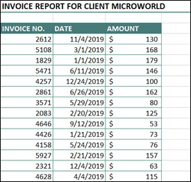
For instance, imagine reconciling invoices. You have your list and the client’s list. Using VLOOKUP, you can quickly pinpoint missing invoices without manual cross-referencing.
Key Considerations Before Using VLOOKUP
- Unique Identifier: Each record in both lists must have a unique identifier (e.g., invoice number, product ID). VLOOKUP uses this identifier to match entries. While other data points might exist, a unique identifier is crucial for accurate comparison.
- Uniqueness of the Lookup Value: The lookup value (the identifier you’re searching for) must be unique within the lookup table. Duplicate values can lead to incorrect results. Always verify the uniqueness of your chosen identifier.
- Lookup Value in the First Column: VLOOKUP searches in the first column of the lookup table. Ensure your unique identifier resides in the leftmost column of your comparison data.
- Duplicate Check: Before applying VLOOKUP, check for duplicate values in the column containing the lookup value. This prevents erroneous matches and ensures accurate comparison results.
Step-by-Step Guide: Comparing Lists with VLOOKUP
1. Naming the Range
To simplify your formula, name the range containing the lookup table.
- Select the entire data range in your lookup table (e.g., the client’s invoice list).
- In the Name Box (top left corner of Excel), enter a descriptive name (e.g., “ClientInvoices”) and press Enter.
2. Constructing the VLOOKUP Formula
The VLOOKUP function consists of four arguments:
VLOOKUP(lookup_value, table_array, col_index_num, [range_lookup])
lookup_value: The cell containing the value you want to search for in the lookup table. This will be the unique identifier in your main list.table_array: The named range or cell range of your lookup table (e.g., “ClientInvoices”).col_index_num: Since we are only checking for the existence of the item, you can use “1” to return the lookup value itself if found.[range_lookup]: Use “FALSE” (or 0) for an exact match. This is critical for accurate comparisons.
3. Handling Errors with ISNA
VLOOKUP returns #N/A if a value isn’t found. Use the ISNA function to make the results more user-friendly.
=ISNA(VLOOKUP(lookup_value, table_array, col_index_num, FALSE))
This will return “TRUE” if the value is missing and “FALSE” if it’s found.
4. Enhancing Readability with IF
Combine ISNA with the IF function to display more meaningful results:
=IF(ISNA(VLOOKUP(lookup_value, table_array, col_index_num, FALSE)), "Missing Record", "")
This formula displays “Missing Record” if the item isn’t found and leaves the cell blank if it is.
5. Highlighting Missing Records with Conditional Formatting
- Copy the
ISNA(VLOOKUP(...))portion of your formula. - Select the data range in your main list.
- Go to Home > Conditional Formatting > New Rule > Use a formula to determine which cells to format.
- Paste the copied formula into the formula input box (add an equals sign at the beginning).
- Choose a formatting style to highlight the missing records (e.g., a fill color).
By combining VLOOKUP with ISNA, IF, and Conditional Formatting, you can efficiently compare two lists, clearly identify discrepancies, and enhance the readability of your results. This method significantly streamlines data reconciliation tasks in Excel.