**How Do I Compare Two Columns in Excel for Differences?**

Comparing two columns in Excel for differences is a common task for data analysis. At COMPARE.EDU.VN, we provide clear and effective methods to identify these discrepancies, ensuring data integrity and accuracy. This guide will walk you through various techniques to compare columns, empowering you to streamline your data analysis and decision-making. Discover powerful tools to analyze discrepancies and gain insights.

1. Why Comparing Two Columns in Excel Matters

Excel is a cornerstone for data storage, manipulation, and analysis. When working with large datasets, comparing columns becomes essential.

1.1. The Importance of Data Integrity

Data analysts use Excel to make informed marketing and sales decisions. The integrity of this data is paramount. Comparing columns helps to:

Identify Missing Data: Determine if cells are empty or contain critical information.
Ensure Consistency: Verify data accuracy across multiple spreadsheets linked together.
Save Time: Automate the comparison process instead of manual checks, which can be time-consuming.

1.2. Practical Applications

Consider these scenarios where comparing columns is invaluable:

Inventory Management: Compare stock levels in two different spreadsheets to identify discrepancies.
Customer Data Analysis: Verify customer information across databases to ensure data accuracy.
Financial Audits: Compare transaction records to detect anomalies or errors.
Academic Research: Cross-reference research data to validate findings.

2. Methods to Compare Two Columns in Excel

Several methods exist to compare two columns in Excel, each suited to different needs. Here are some common techniques:

2.1. Using the Equals Operator (=)

The equals operator provides a simple, row-by-row comparison. It returns TRUE if the values match and FALSE if they don’t.

2.1.1. Step-by-Step Guide

Select a Cell: In a new column, select the first cell next to the rows you want to compare (e.g., C2).
Enter the Formula: Type =A2=B2 and press Enter. This formula compares the values in cells A2 and B2.
Drag Down: Drag the fill handle (the small square at the bottom-right of the cell) down to apply the formula to the rest of the rows.

2.1.2. Interpreting the Results

TRUE: The values in the compared rows are identical.
FALSE: The values are different.

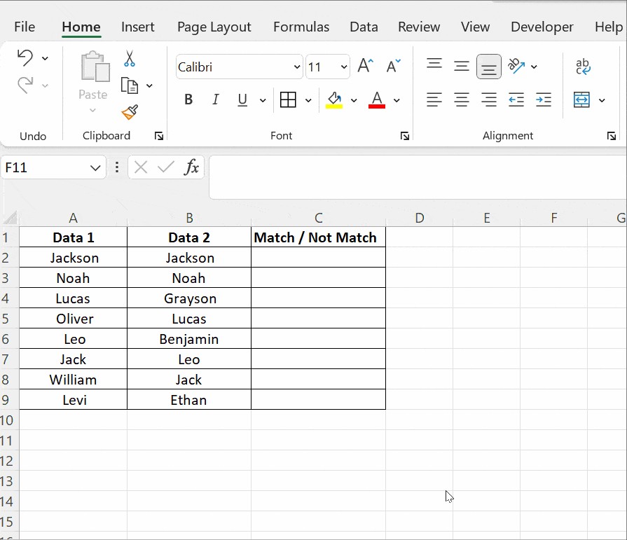
2.2. Using the IF Condition

The IF condition enhances the comparison by allowing you to display custom messages like “Match” or “Not Match.”

2.2.1. Basic IF Formula

The formula =IF(A2=B2,"Match"," ") returns “Match” if the values in A2 and B2 are the same, and leaves the cell blank if they are different.

2.2.2. Identifying Mismatches

To specifically identify mismatches, use the formula =IF(A2=B2,"Match","Not a Match"). This formula returns “Not a Match” when the values differ.

2.2.3. Comparing for Differences

To compare for differences specifically, replace the equals sign with the not-equal-to sign (<>): =IF(A2<>B2,"Match","Not a Match").

2.3. Using the EXACT() Function

The EXACT() function performs a case-sensitive comparison. This is useful when distinguishing between uppercase and lowercase letters is crucial.

2.3.1. Syntax

The syntax is =EXACT(text1, text2). It returns TRUE if the text strings are identical (including case) and FALSE otherwise.

2.3.2. Example

Consider two cells: A2 contains “Nova Scotia” and B2 contains “nova scotia.”

=IF(A2=B2, "Match", "Mismatch") would return “Match” because the equals operator is case-insensitive.
=IF(EXACT(A2, B2), "Match", "Mismatch") would return “Mismatch” because the EXACT() function is case-sensitive.

2.4. Using Conditional Formatting

Conditional formatting visually highlights unique or duplicate values, making differences immediately apparent.

2.4.1. Highlighting Duplicate Values

Select Columns: Choose the columns you want to compare.
Go to Conditional Formatting: Click Home → Styles → Conditional Formatting → Highlight Cells Rules → Duplicate Values.
Choose Formatting: Select how you want to highlight the duplicate values (e.g., fill with color, change text color).

2.4.2. Highlighting Unique Values

Follow the same steps, but in the Duplicate Values dialog box, choose “Unique” instead of “Duplicate.”

2.4.3. Clearing Formatting

To remove conditional formatting, click Conditional Formatting → Clear Rules → Clear Rules from Selected Cells.

2.5. Using Lookup Functions

Lookup functions, like VLOOKUP, HLOOKUP, and XLOOKUP, are powerful tools for comparing data across columns or tables.

2.5.1. VLOOKUP Example

Suppose column A lists exams taken by students, and column B lists subjects they passed. Use VLOOKUP to identify which exams were passed.

Enter the Formula: In cell C2, enter =VLOOKUP(A2, $B$2:$B$5, 1, 0).
Drag Down: Apply the formula to the rest of the rows in column C.

2.5.2. Understanding the Formula

VLOOKUP(A2, $B$2:$B$5, 1, 0): This function searches for the value in A2 within the range B2:B5. The $ symbols create an absolute reference, ensuring the range doesn’t change when you drag the formula down. The “1” indicates that the value should be returned from the first column in the range, and “0” specifies an exact match.

2.5.3. Interpreting the Results

Value Returned: If a subject in column A is found in column B, the function returns that subject.
#N/A: If a subject in column A is not found in column B, the function returns #N/A, indicating it was not cleared.

3. Detailed Steps and Advanced Techniques

For a deeper understanding, let’s explore detailed steps and advanced techniques for comparing columns in Excel.

3.1. Comprehensive Use of the IF Condition

The IF condition is versatile and can be adapted for more complex comparisons.

3.1.1. Nested IF Statements

Nested IF statements allow for multiple conditions within a single formula.

Example: =IF(A2=B2, "Match", IF(A2>B2, "A is Greater", "B is Greater"))
Explanation: This formula first checks if A2 equals B2. If true, it returns “Match.” If false, it checks if A2 is greater than B2. If true, it returns “A is Greater”; otherwise, it returns “B is Greater.”

3.1.2. Using AND and OR with IF

The AND and OR functions can combine multiple conditions in an IF statement.

Example (AND): =IF(AND(A2=B2, C2=D2), "Full Match", "Partial or No Match")
Explanation: This formula checks if both A2 equals B2 AND C2 equals D2. If both are true, it returns “Full Match”; otherwise, it returns “Partial or No Match.”
Example (OR): =IF(OR(A2=B2, C2=D2), "At Least One Match", "No Match")
Explanation: This formula checks if either A2 equals B2 OR C2 equals D2. If either is true, it returns “At Least One Match”; otherwise, it returns “No Match.”

3.2. Advanced Conditional Formatting Techniques

Conditional formatting can be customized to highlight specific differences.

3.2.1. Using Formulas in Conditional Formatting

Select Columns: Choose the columns you want to compare.
Go to Conditional Formatting: Click Home → Styles → Conditional Formatting → New Rule.
Select Rule Type: Choose “Use a formula to determine which cells to format.”
Enter the Formula: Enter a formula that returns TRUE for the cells you want to highlight. For example, to highlight cells in column A that are not in column B, you might use =ISNA(MATCH(A1, $B:$B, 0)).
Format: Click “Format” and choose your desired formatting (e.g., fill color).

3.2.2. Explaining the Formula

MATCH(A1, $B:$B, 0): This function searches for the value in A1 within the entire column B. If it finds a match, it returns the row number; otherwise, it returns #N/A.
ISNA(...): This function checks if the result of the MATCH function is #N/A. If it is, it returns TRUE; otherwise, it returns FALSE.
By combining these functions, you can highlight cells in column A that do not have a corresponding match in column B.

3.3. In-Depth Look at Lookup Functions

Lookup functions are essential for comparing data across large datasets.

3.3.1. HLOOKUP

HLOOKUP (Horizontal Lookup) searches for a value in the top row of a table and returns a value in the same column from a row you specify.

Syntax: HLOOKUP(lookup_value, table_array, row_index_num, [range_lookup])
Example: =HLOOKUP("Product Code", A1:E10, 2, FALSE)
Explanation: This formula searches for “Product Code” in the top row of the range A1:E10 and returns the value from the second row in the same column. FALSE specifies an exact match.

3.3.2. XLOOKUP

XLOOKUP is a modern lookup function that combines the capabilities of VLOOKUP and HLOOKUP with added flexibility.

Syntax: XLOOKUP(lookup_value, lookup_array, return_array, [if_not_found], [match_mode], [search_mode])
Example: =XLOOKUP(A2, $B$2:$B$5, $C$2:$C$5, "Not Found", 0)
Explanation: This formula searches for the value in A2 within the range B2:B5 and returns the corresponding value from the range C2:C5. If the value is not found, it returns “Not Found.” The “0” specifies an exact match.

3.3.3. INDEX-MATCH

The INDEX-MATCH combination is a powerful alternative to VLOOKUP, offering more flexibility.

MATCH Function:
- Syntax: MATCH(lookup_value, lookup_array, [match_type])
- Purpose: Finds the position of a value in an array.
INDEX Function:
- Syntax: INDEX(array, row_num, [column_num])
- Purpose: Returns the value at a specific position in an array.

3.3.4. Example

Suppose you want to find the name of a product in column B based on its product code in column A. You can use the following formula:

=INDEX($B$2:$B$10, MATCH(A2, $A$2:$A$10, 0))
Explanation:
- MATCH(A2, $A$2:$A$10, 0): This finds the position of the product code in A2 within the range A2:A10.
- INDEX($B$2:$B$10, ...): This returns the value from the range B2:B10 at the position found by the MATCH function.

4. Practical Examples and Use Cases

To solidify your understanding, let’s explore real-world examples of comparing columns in Excel.

4.1. Inventory Management

Consider two spreadsheets:

Sheet 1: Contains current inventory levels.
Sheet 2: Contains expected inventory levels.

You want to identify discrepancies between the two.

4.1.1. Steps

Import Data: Ensure both spreadsheets are open in Excel.
Use VLOOKUP: In Sheet 1, add a new column and use VLOOKUP to compare the inventory levels with Sheet 2.
- =VLOOKUP(A2, 'Sheet2'!$A$2:$B$100, 2, FALSE)
- Explanation: This formula searches for the product code in A2 within the range A2:B100 in Sheet 2 and returns the inventory level from the second column.
Use IF Condition: Add another column to identify discrepancies.
- =IF(B2=C2, "Match", "Discrepancy")
- Explanation: This formula compares the inventory level in Sheet 1 (B2) with the inventory level retrieved from Sheet 2 (C2) and indicates if there is a discrepancy.
Conditional Formatting: Highlight the discrepancies for quick identification.

4.1.2. Benefits

Quickly identify inventory discrepancies.
Reduce manual errors.
Improve inventory accuracy.

4.2. Customer Data Analysis

Suppose you have two customer databases:

Database 1: Contains customer information from the past year.
Database 2: Contains updated customer information.

You want to identify which customers have updated their information.

4.2.1. Steps

Import Data: Open both databases in Excel.
Use INDEX-MATCH: In Database 1, add columns to retrieve updated information from Database 2.
- =INDEX('Database2'!$B$2:$B$100, MATCH(A2, 'Database2'!$A$2:$A$100, 0))
- Explanation: This formula searches for the customer ID in A2 within Database 2 and returns the corresponding name.
Compare Data: Use the IF condition to compare the information.
- =IF(B2=C2, "No Change", "Updated")
- Explanation: This formula compares the customer name in Database 1 (B2) with the customer name retrieved from Database 2 (C2) and indicates if the information has been updated.
Filter Data: Filter the data to view only the customers who have updated their information.

4.2.2. Benefits

Efficiently identify updated customer information.
Improve data accuracy.
Enhance customer relationship management.

4.3. Financial Audits

Consider comparing two sets of financial records:

Record Set 1: Contains transaction data from the bank.
Record Set 2: Contains internal transaction records.

You need to identify any discrepancies between the two.

4.3.1. Steps

Import Data: Open both record sets in Excel.
Use VLOOKUP: In Record Set 1, add columns to compare with Record Set 2.
- =VLOOKUP(A2, 'Record Set 2'!$A$2:$C$100, 3, FALSE)
- Explanation: This formula searches for the transaction ID in A2 within Record Set 2 and returns the transaction amount.
Compare Data: Use the IF condition to compare the amounts.
- =IF(B2=C2, "Match", "Discrepancy")
- Explanation: This formula compares the transaction amount in Record Set 1 (B2) with the amount retrieved from Record Set 2 (C2) and indicates if there is a discrepancy.
Conditional Formatting: Highlight the discrepancies for easy identification.

4.3.2. Benefits

Efficiently identify financial discrepancies.
Improve audit accuracy.
Enhance financial compliance.

5. Addressing Common Challenges

While comparing columns in Excel, you may encounter some challenges. Here’s how to tackle them:

5.1. Different Data Types

Ensure that the data types in both columns are consistent. For example, if one column contains numbers and the other contains text, the comparison may not work correctly.

Solution: Use the VALUE() function to convert text to numbers or the TEXT() function to convert numbers to text.

5.2. Extra Spaces

Extra spaces can cause discrepancies.

Solution: Use the TRIM() function to remove extra spaces from the data.

5.3. Case Sensitivity

The equals operator (=) is case-insensitive.

Solution: Use the EXACT() function for case-sensitive comparisons.

5.4. Error Values

Error values like #N/A can disrupt comparisons.

Solution: Use the IFERROR() function to handle error values.

5.5. Large Datasets

Comparing very large datasets can be slow.

Solution: Use Excel’s built-in tools like Power Query to efficiently compare large datasets.

6. Best Practices for Comparing Columns in Excel

Follow these best practices to ensure accurate and efficient comparisons:

6.1. Clean Your Data

Before comparing, clean your data by removing extra spaces, correcting data types, and handling error values.

6.2. Use Helper Columns

Use helper columns to break down complex comparisons into smaller, more manageable steps.

6.3. Validate Your Formulas

Double-check your formulas to ensure they are correct and accurate.

6.4. Use Named Ranges

Use named ranges to make your formulas more readable and easier to understand.

6.5. Document Your Process

Document your comparison process so that others can easily understand and replicate it.

7. Frequently Asked Questions (FAQ)

Q1: How can I compare two columns in Excel and highlight the differences?

Use conditional formatting with a formula. Select the columns, go to “Conditional Formatting,” choose “New Rule,” and use a formula like =A1<>B1 to highlight the differences.

Q2: What is the difference between VLOOKUP and XLOOKUP?

VLOOKUP searches for a value in the first column of a range, while XLOOKUP offers more flexibility by allowing you to specify the lookup and return arrays separately. XLOOKUP also handles errors more gracefully.

Q3: How can I compare two columns in different Excel sheets?

Use formulas like VLOOKUP or INDEX-MATCH, referencing the columns in the other sheet by including the sheet name in the formula (e.g., =VLOOKUP(A2, 'Sheet2'!$A$2:$B$100, 2, FALSE)).

Q4: Can I compare two columns for partial matches?

Yes, you can use functions like SEARCH or FIND within an IF statement to check for partial matches. For example, =IF(ISNUMBER(SEARCH(A1, B1)), "Partial Match", "No Match").

Q5: How do I compare two columns and return a value from a third column?

Use a combination of IF and VLOOKUP. First, compare the two columns using IF, and if they match, use VLOOKUP to return a value from the third column. For example, =IF(A2=B2, VLOOKUP(A2, $D$2:$E$100, 2, FALSE), "No Match").

Q6: What is the best way to compare two very large columns in Excel?

For large datasets, consider using Power Query, which is designed to handle large amounts of data efficiently.

Q7: How can I ignore case sensitivity when comparing two columns?

Use the UPPER or LOWER functions to convert both columns to the same case before comparing. For example, =IF(UPPER(A2)=UPPER(B2), "Match", "No Match").

Q8: How do I compare two columns and count the number of matches?

Use the COUNTIF function. For example, to count the number of matches in column B with values in column A, use =COUNTIF(B:B, A1). Drag this formula down to apply it to all rows.

Q9: Can I use VBA to compare two columns in Excel?

Yes, VBA can be used to compare two columns, especially for complex scenarios. You can write a VBA macro to loop through the rows and compare the values.

Q10: How do I compare two columns and list the differences?

Use a combination of IF, ISNA, and MATCH. The formula =IF(ISNA(MATCH(A1, $B:$B, 0)), A1, "") will list the values in column A that are not found in column B.

8. Conclusion: Streamline Your Data Analysis with Effective Column Comparisons

Comparing two columns in Excel is a fundamental skill for data analysis, helping you ensure data integrity, identify discrepancies, and make informed decisions. By mastering the techniques outlined in this guide, you can streamline your workflow and gain deeper insights from your data. Whether you’re managing inventory, analyzing customer data, or conducting financial audits, these methods will empower you to work more efficiently and accurately.

At COMPARE.EDU.VN, we understand the importance of making informed decisions based on reliable data. That’s why we offer comprehensive comparisons of various products, services, and ideas.

Ready to make smarter decisions? Visit COMPARE.EDU.VN to find detailed, objective comparisons that help you choose the best option for your needs. Don’t leave your decisions to chance; let us help you compare and decide with confidence.

Contact Us:

Address: 333 Comparison Plaza, Choice City, CA 90210, United States
WhatsApp: +1 (626) 555-9090
Website: COMPARE.EDU.VN

Start comparing today and make better choices with compare.edu.vn!