How Do I Compare Two Columns In Excel? A Comprehensive Guide

How Do I Compare 2 Columns In Excel efficiently and accurately? COMPARE.EDU.VN provides a detailed guide to help you master this essential skill. Learn to identify matches, differences, and unique values within your data, enhancing your analysis and decision-making with effective comparison techniques and practical examples. Explore various methods to streamline your data analysis workflow with our in-depth walkthrough.

1. Why Comparing Two Columns in Excel is Essential

Excel, a powerhouse for data storage, manipulation, and informed decision-making, is a crucial tool for data analysis. Its versatility allows users to extract meaningful insights. Data analysts use Excel to gather information that significantly impacts marketing and sales strategies.

The absence of data in a cell, depending on the applied formulas or tools, can have significant implications. Excel spreadsheets can be extensive, and multiple spreadsheets are often interconnected. In these scenarios, data analysts frequently need to compare two columns within the same or different spreadsheets. Manually comparing columns is a time-consuming and laborious process, potentially taking hours or even days to identify missing data.

Comparing two columns in Excel is essential for data analysts to ascertain whether a cell contains data or not. The results of these comparisons are typically displayed as TRUE/FALSE, Match/Not Match, or custom user-defined messages, providing immediate feedback on data integrity. This detailed comparison helps identify discrepancies and ensures data accuracy, which is vital for reliable analysis and strategic decision-making.

2. Effective Methods to Compare Two Columns in Excel

When managing data across different columns, tables, or spreadsheets, the ability to compare data is essential for identifying missing information or verifying consistency. The best method for comparison will depend on your specific analytical goals. Below are several efficient strategies to compare two columns in Excel:

Using functions to highlight unique or duplicate values in each column.
Employing conditional formatting or formulas to display unique or duplicate entries.
Conducting row-by-row comparisons.
Utilizing LOOKUP formulas.

2.1. Comparing Two Columns Using the Equals Operator

You can compare data row by row to find matching data, returning results as “Match” or “Not Match.” For example, the formula =A2=B2 identifies matching data and returns “True” or “False.” This method provides a straightforward way to assess data alignment across columns.

To implement this comparison, enter the formula in cell C2 and drag it down to the end of the table. The formula returns “TRUE” if the values in the compared rows are identical and “FALSE” if they differ. This method is useful for quickly identifying discrepancies and ensuring data consistency across your spreadsheet.

2.2. Using the IF Condition to Compare Two Columns

In Excel, you can use the IF condition to compare two columns. The formula =IF(A2=B2,"Match"," ") returns “Match” for rows with matching values, leaving the other rows blank. This approach clearly indicates which rows contain identical entries.

The same formula can also identify and display mismatching values. You can modify the IF condition to show a specific result when the condition is false. For instance, the formula =IF(A2=B2,"Match","Not a Match") returns “Match” for identical values and “Not a Match” for differences.

To compare columns and specifically highlight differences, replace the equals sign with the non-equality sign (<>). The formula =IF(A2<>B2,"Match","Not a Match") will return “Match” when values differ and “Not a Match” when they are the same.

Using the IF condition provides a versatile way to compare two columns, allowing you to identify both matches and mismatches based on your specific criteria. This method is effective for data validation and ensuring accuracy in your spreadsheets.

2.3. Comparing Two Columns with the EXACT() Function

When you need to compare two columns in Excel and want to consider case sensitivity, the EXACT() function is invaluable.

The EXACT() function compares two text strings and returns TRUE if they are identical, including case, and FALSE otherwise. It is case-sensitive but ignores formatting differences. The syntax is =EXACT(text1, text2), where both text1 and text2 are required arguments.

Consider an example where columns A and B contain the text strings “Nova Scotia” in different cases.

Applying the formula =IF(A2=B2, "Match", "Mismatch") to cell C2 returns “Match” because this comparison is case-insensitive.

To enforce case sensitivity, use the formula =IF(EXACT(A2, B2), "Match", "Mismatch").

The EXACT() function returns either TRUE or FALSE, which the IF condition then uses to determine the final output. The IF condition evaluates the result and returns the first argument if TRUE and the second argument if FALSE.

2.4. Using Conditional Formatting to Compare Two Columns

To use conditional formatting, go to Home, then Styles, and select Conditional Formatting → Highlight Cell Rules → Duplicate Values. A dialogue box will appear, allowing you to choose the values from a drop-down menu.

Apply the formatting condition to the selected cells. You can choose to highlight either Duplicate or Unique values.
Specify the format for the cells that meet the condition, such as filling with a color, changing the text color, or altering the cell border.

For example, consider two data sets in columns Data1 and Data2, where not all names in Data1 are present in Data2. To find and highlight the names that appear in both columns, select the entire table and follow the steps above. Choose Duplicate to highlight common names and select a formatting option like filling the cell with color, changing the text color, or modifying the cell border.

For a custom color not listed in the drop-down menu, choose Custom Format.

Alternatively, use the Unique option to highlight cells containing data that is not repeated. This option is useful for identifying unique entries in your columns.

To clear the formatting applied to the cells, select Conditional Formatting → Clear Rules → Clear Rules from Selected Cells.

Conditional formatting is useful when you don’t want to add a third column to show comparison results. You can highlight duplicate (matching) and unique (different) data to show which rows have the same data, or use an additional column to display values indicating whether the data matches. While effective for smaller tables, larger spreadsheets may require more complex methods.

2.5. Utilizing Lookup Functions to Compare Two Columns

The LOOKUP function searches for a specified value in a row or column and returns a corresponding value from another row or column. Key lookup functions include HLOOKUP, VLOOKUP, and XLOOKUP. The letters H and V stand for horizontal and vertical, respectively, and XLOOKUP combines the functionalities of both LOOKUP and VLOOKUP.

For example, to compare two columns using VLOOKUP():

Column A lists exams taken by a student, and column B lists subjects the student passed. The result sheet should list all subjects, with VLOOKUP() applied in cell C2 as =VLOOKUP(A2, $B$2:$B$5,1,0).

Drag the formula down to apply it to all cells below C2. Column C will show the cleared subjects, while those not cleared will appear as #N/A. The formula elements include:

VLOOKUP(A2,..,..,..): Takes the value in cell A2.
VLOOKUP(A2, $B$2:$B$5,..,..): Compares with values in cells B2 to B5, using absolute references ($ symbol) to lock the range.
VLOOKUP(A2, $B$2:$B$5,1,..): Specifies the column index number, indicating the position of the column to compare from the lookup value A2. In this case, the subjects list is in column A, and the comparison column is 1 column away, hence the value 1.
VLOOKUP(A2, $B$2:$B$5,1,0): The last argument is a logical value (0 or 1). Use 0 to find an exact match or 1 to return the closest match sorted in ascending order.

3. Streamlining Data Comparison with Advanced Techniques

Beyond basic methods, Excel offers advanced techniques to handle complex data comparisons. These techniques allow for more precise analysis and efficient data management, particularly when dealing with large datasets or specific comparison criteria.

3.1. Combining INDEX-MATCH for Flexible Lookups

While VLOOKUP is commonly used, the INDEX-MATCH function provides a more flexible and powerful alternative for comparing and retrieving data across tables. This combination allows you to look up values based on row and column matches, even when the lookup and return columns are not adjacent.

INDEX: Returns the value of a cell in a table based on the row and column number.
MATCH: Searches for a value in a row or column and returns the position of that item.

By combining these functions, you can perform lookups in any direction and handle more complex scenarios where VLOOKUP might fall short.

3.2. Utilizing Array Formulas for Complex Comparisons

Array formulas allow you to perform calculations on multiple values in one or more arrays. These are particularly useful for comparing ranges of data that do not align neatly in rows or columns. To enter an array formula, you must press Ctrl + Shift + Enter.

For example, you can use an array formula to compare two columns and return the number of matching values:

=SUM(IF(A1:A10=B1:B10,1,0))

This formula compares each cell in the range A1:A10 with the corresponding cell in B1:B10. If the values match, it assigns 1; otherwise, it assigns 0. The SUM function then adds up all the 1s, giving you the total number of matches.

3.3. Employing Pivot Tables for Summary Comparisons

Pivot tables are powerful tools for summarizing and analyzing data, including comparing data across two columns. You can use pivot tables to group and count data from two columns to identify patterns and discrepancies.

To compare two columns using a pivot table:

Select your data range.
Go to Insert and click PivotTable.
In the PivotTable Fields pane, drag one column to the Rows area and the other to the Columns area.
Drag one of the columns to the Values area and set the calculation to Count.

The resulting pivot table will show a summary of how the values in the two columns relate to each other, making it easy to spot similarities and differences.

4. Practical Applications of Column Comparison in Excel

Comparing columns in Excel is not just a theoretical exercise; it has numerous practical applications across various fields. Understanding these applications can help you leverage Excel more effectively in your daily tasks.

4.1. Data Validation and Cleaning

One of the primary uses of column comparison is to validate and clean data. When dealing with large datasets, errors and inconsistencies are inevitable. By comparing columns, you can identify and correct these issues, ensuring data accuracy and reliability.

Identifying Duplicates: Use conditional formatting or formulas to find duplicate entries, which can then be reviewed and removed.
Verifying Data Integrity: Compare data entered from different sources to ensure consistency and accuracy.
Spotting Errors: Quickly identify discrepancies between columns that should contain identical data.

4.2. Financial Analysis

In financial analysis, comparing columns is crucial for tasks such as reconciliation, budgeting, and auditing.

Reconciliation: Compare bank statements with internal records to identify discrepancies and ensure all transactions are accounted for.
Budgeting: Compare actual expenses with budgeted amounts to track performance and identify areas where adjustments are needed.
Auditing: Compare data from different periods to detect anomalies and potential fraud.

4.3. Sales and Marketing

Sales and marketing teams can use column comparison to analyze customer data, track campaign performance, and optimize strategies.

Customer Data Analysis: Compare customer lists from different sources to identify overlaps and gaps in your customer base.
Campaign Tracking: Compare data from different marketing campaigns to determine which strategies are most effective.
Sales Performance: Compare sales data across different regions or time periods to identify trends and opportunities.

4.4. Inventory Management

Effective inventory management relies on accurate data. Comparing columns can help track inventory levels, identify discrepancies, and prevent stockouts or overstocking.

Stock Level Tracking: Compare physical inventory counts with recorded levels to identify discrepancies.
Order Management: Compare order data with shipment data to ensure all orders are fulfilled accurately.
Supply Chain Analysis: Compare data from different suppliers to identify the most reliable and cost-effective sources.

5. Common Challenges and Solutions

While comparing columns in Excel is a powerful tool, it can present certain challenges. Understanding these challenges and knowing how to address them can help you avoid common pitfalls and ensure accurate results.

5.1. Dealing with Large Datasets

Comparing large datasets can be slow and resource-intensive. Excel may become sluggish, and formulas may take a long time to calculate.

Solution: Use Excel’s built-in features like filtering and sorting to reduce the dataset size. Consider using array formulas or pivot tables, which are optimized for handling large amounts of data. Alternatively, you can use database software like SQL for more efficient data processing.

5.2. Handling Different Data Types

Comparing columns with different data types (e.g., text and numbers) can lead to inaccurate results. Excel may not recognize matches correctly if the data types are inconsistent.

Solution: Use the TEXT function to convert numbers to text or the VALUE function to convert text to numbers. Ensure that the data types are consistent before performing the comparison.

5.3. Managing Case Sensitivity

Excel formulas are generally case-insensitive, which can be problematic when comparing text data where case matters.

Solution: Use the EXACT function for case-sensitive comparisons. This function returns TRUE only if the text strings are identical, including case.

5.4. Addressing Errors and Inconsistencies

Errors and inconsistencies in your data can skew comparison results. This includes typos, missing values, and inconsistent formatting.

Solution: Use Excel’s data validation tools to enforce data entry rules and minimize errors. Clean your data by removing duplicates, correcting typos, and standardizing formatting. Use formulas like TRIM to remove extra spaces and CLEAN to remove non-printable characters.

5.5. Coping with Complex Criteria

Sometimes, simple comparisons are not enough. You may need to compare columns based on multiple criteria or conditions.

Solution: Use nested IF statements or more advanced functions like SUMIFS and COUNTIFS to handle complex criteria. These functions allow you to specify multiple conditions for your comparisons.

6. Advanced Excel Functions for Column Comparison

To maximize the efficiency and accuracy of comparing columns in Excel, consider leveraging these advanced functions:

6.1. OFFSET Function

The OFFSET function returns a range of cells that is a specified number of rows and columns from a starting cell. This is useful when you need to compare data that is not in adjacent columns.

Syntax: =OFFSET(reference, rows, cols, [height], [width])

reference: The starting cell.
rows: The number of rows to offset.
cols: The number of columns to offset.
[height]: The height of the returned range (optional).
[width]: The width of the returned range (optional).

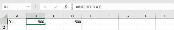
6.2. INDIRECT Function

The INDIRECT function returns the reference specified by a text string. This allows you to create dynamic references that can change based on cell values.

Excel INDIRECT function

Syntax: =INDIRECT(ref_text, [a1])

ref_text: A text string that refers to a cell.
[a1]: A logical value specifying whether ref_text contains an A1-style or R1C1-style reference. If omitted, it is assumed to be A1-style.

6.3. AGGREGATE Function

The AGGREGATE function can apply different aggregate functions (like SUM, AVERAGE, COUNT) to a list or database, with the option to ignore errors and hidden rows.

Syntax: =AGGREGATE(function_num, options, ref1, [ref2], ...)

function_num: A number specifying the aggregate function to use.
options: A number specifying which values to ignore.
ref1, [ref2], ...: The range of cells to aggregate.

7. Optimizing Your Excel Skills for Data Analysis

Mastering Excel for data analysis requires continuous learning and skill development. Here are some tips to help you optimize your Excel skills:

Take Online Courses: Websites like Coursera, Udemy, and LinkedIn Learning offer comprehensive Excel courses that cover everything from basic to advanced topics.
Practice Regularly: The more you use Excel, the more comfortable you will become with its features and functions. Practice with real-world datasets to hone your skills.
Explore Excel Templates: Microsoft offers a variety of Excel templates for different tasks, such as budgeting, project management, and data analysis. These templates can provide inspiration and help you learn new techniques.
Join Online Communities: Engage with other Excel users on forums and social media groups. Sharing tips and tricks can help you learn new ways to use Excel and stay up-to-date with the latest features.
Read Excel Blogs and Articles: Many websites and blogs offer tutorials, tips, and tricks for using Excel. Subscribe to these resources to stay informed and improve your skills.
Attend Workshops and Seminars: Consider attending Excel workshops and seminars to learn from experts and network with other users.
Customize Your Ribbon: Add frequently used commands to your Excel ribbon for quick access. This can save time and streamline your workflow.
Learn Keyboard Shortcuts: Mastering keyboard shortcuts can significantly speed up your work in Excel. Create a cheat sheet of common shortcuts and keep it handy.
Use Named Ranges: Assign names to cells or ranges of cells to make your formulas more readable and easier to understand.
Automate Repetitive Tasks: Use macros to automate repetitive tasks and save time. Learn VBA (Visual Basic for Applications) to create custom macros that meet your specific needs.
Validate Your Data: Use data validation tools to enforce data entry rules and minimize errors. This can improve the accuracy and reliability of your data.
Visualize Your Data: Use charts and graphs to visualize your data and make it easier to understand. Experiment with different chart types to find the best way to present your data.

By implementing these tips, you can enhance your Excel skills and become a more proficient data analyst. Remember that continuous learning and practice are key to mastering Excel and unlocking its full potential.

8. Frequently Asked Questions

8.1. How can I compare two columns in Excel to find differences?

To find differences between two columns, use the formula =IF(A2<>B2, "Different", "Same"). This formula compares the values in cells A2 and B2 and returns “Different” if they are not equal, and “Same” if they are equal. Drag the formula down to apply it to all rows in your data.

8.2. Is it possible to compare two columns in different Excel sheets?

Yes, you can compare columns in different sheets by referencing the sheet name in your formula. For example, to compare column A in Sheet1 with column A in Sheet2, use the formula =IF(Sheet1!A2=Sheet2!A2, "Match", "No Match") in a third sheet.

8.3. How do I highlight matching values in two columns?

Use conditional formatting to highlight matching values. Select both columns, go to Home → Conditional Formatting → Highlight Cells Rules → Duplicate Values, and choose “Duplicate” from the drop-down menu. This will highlight all values that appear in both columns.

8.4. Can I compare two columns and return a value from a third column?

Yes, you can use the INDEX and MATCH functions to compare two columns and return a value from a third column. For example, if you want to compare column A and column B, and return the corresponding value from column C when there is a match, use the formula =INDEX(C:C, MATCH(A2, B:B, 0)).

8.5. What is the best way to compare two columns for case-sensitive matches?

Use the EXACT function for case-sensitive comparisons. The formula =IF(EXACT(A2, B2), "Match", "No Match") will compare the values in cells A2 and B2, considering case, and return “Match” only if they are identical.

8.6. How can I compare two columns and count the number of matches?

Use the SUM and IF functions to count the number of matches. The array formula =SUM(IF(A1:A10=B1:B10, 1, 0)) compares the values in the ranges A1:A10 and B1:B10 and returns the total number of matches. Remember to enter this formula by pressing Ctrl + Shift + Enter.

8.7. How do I compare two columns and identify unique values?

Use conditional formatting to highlight unique values. Select both columns, go to Home → Conditional Formatting → Highlight Cells Rules → Duplicate Values, and choose “Unique” from the drop-down menu. This will highlight all values that appear only once across both columns.

8.8. Can I compare two columns based on multiple criteria?

Yes, use nested IF statements or functions like SUMIFS or COUNTIFS to compare columns based on multiple criteria. These functions allow you to specify multiple conditions for your comparisons.

8.9. How can I handle errors when comparing two columns?

Use the IFERROR function to handle errors that may occur during the comparison. For example, if you are using VLOOKUP and want to return a specific value when no match is found, use the formula =IFERROR(VLOOKUP(A2, B:C, 2, FALSE), "Not Found").

8.10. What are the best practices for comparing columns in large datasets?

For large datasets, use Excel’s built-in features like filtering and sorting to reduce the dataset size. Consider using array formulas or pivot tables, which are optimized for handling large amounts of data. Additionally, ensure that your data is clean and consistent to avoid errors.

9. Conclusion

Comparing two columns in Excel is a fundamental skill for data analysis, offering numerous methods to match and compare data across single and multiple columns, as well as different spreadsheets. This guide has shown several effective techniques to compare columns for matches and differences.

To further enhance your Excel proficiency, explore advanced functions such as INDEX-MATCH, OFFSET, and INDIRECT, which are essential for handling complex comparisons and data manipulation. These functions, along with best practices for data cleaning and error handling, will empower you to tackle a wide range of data analysis challenges.

Remember, COMPARE.EDU.VN is your trusted resource for objective comparisons and informed decision-making. Visit our website at COMPARE.EDU.VN to explore more in-depth tutorials and resources. Our goal is to help you make the most of your data analysis efforts.

Need more assistance? Contact us at 333 Comparison Plaza, Choice City, CA 90210, United States, or reach out via Whatsapp at +1 (626) 555-9090. We’re here to support your journey to becoming an Excel expert!

Now that you’re equipped with the knowledge and tools to compare columns in Excel efficiently, visit compare.edu.vn today and unlock a world of comparative insights that will empower you to make better decisions!