Excel How to Compare Two Columns: Simple Methods to Find Matches and Differences

Data analysis often requires meticulous comparison of data sets, and when working with Excel, comparing two columns is a fundamental task. Whether you need to identify matching entries, find unique values, or pinpoint differences, Excel offers a variety of powerful tools and formulas to streamline this process. Manually comparing columns, especially in large datasets, can be time-consuming and prone to errors. Fortunately, Excel provides several efficient methods that can accomplish this task in seconds, saving you valuable time and improving accuracy.

This guide will walk you through various techniques to compare two columns in Excel, ranging from simple built-in features to more advanced formulas. By the end of this article, you’ll be equipped with the knowledge to choose the best method for your specific needs and confidently compare columns like a pro.

Understanding Column Comparison in Excel

At its core, comparing columns in Excel involves examining corresponding cells in two columns to determine if they are the same or different. This can be used for various purposes, such as:

• Data Validation: Ensuring data consistency across different lists or datasets.
• Identifying Duplicates: Finding common entries in two columns.
• Finding Unique Values: Identifying entries that exist in one column but not the other.
• Change Tracking: Detecting modifications between two versions of a dataset.
• Data Cleaning: Identifying and correcting inconsistencies in your data.

Excel provides several methods to achieve this, each with its own strengths and best-use cases. Let’s explore these methods in detail.

Effective Methods for Comparing Two Columns in Excel

Here are several proven methods to compare two columns in Excel, catering to different scenarios and levels of complexity:

1. Conditional Formatting for Visual Comparison
2. Equals Operator (=) for Basic Matching
3. VLOOKUP Function for Finding Matches and Differences
4. IF Formula for Customized Results
5. EXACT Formula for Case-Sensitive Comparison

Let’s delve into each of these methods with step-by-step instructions and examples.

1. Conditional Formatting: Visually Highlight Matches and Differences

Conditional formatting is a user-friendly feature in Excel that allows you to apply formatting to cells based on specific criteria. It’s an excellent way to visually identify matches or differences between two columns without writing complex formulas.

Steps to Compare Columns Using Conditional Formatting:

Step 1: Select the Columns

Begin by selecting the two columns you want to compare. You can select entire columns by clicking on the column letters (e.g., ‘A’ and ‘B’) or select specific ranges of cells within the columns.

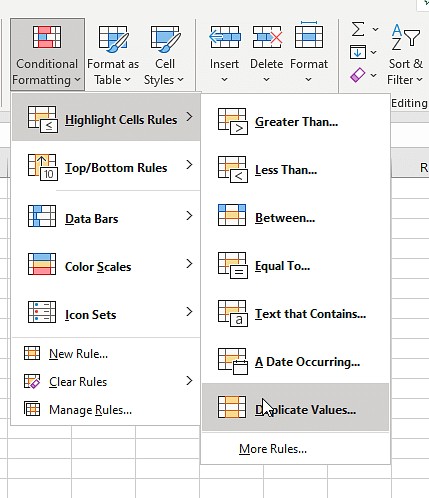
Step 2: Access Conditional Formatting

Navigate to the “Home” tab on the Excel ribbon. In the “Styles” group, click on “Conditional Formatting.”

Step 3: Highlight Duplicate or Unique Values

From the dropdown menu, hover over “Highlight Cells Rules” and then choose either “Duplicate Values…” or “Unique Values…” depending on what you want to highlight.

• Duplicate Values: Highlights cells that appear in both selected columns (matches).
• Unique Values: Highlights cells that appear in only one of the selected columns (differences).

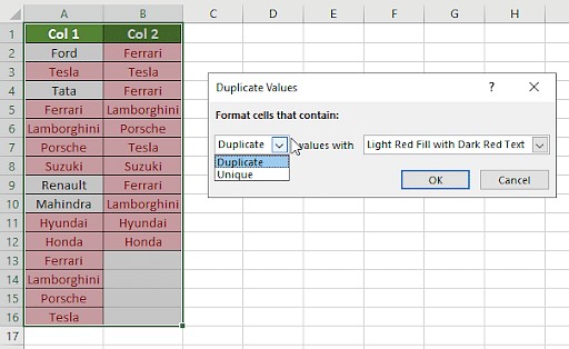
Step 4: Choose Formatting Options

A “Duplicate Values” dialog box will appear.

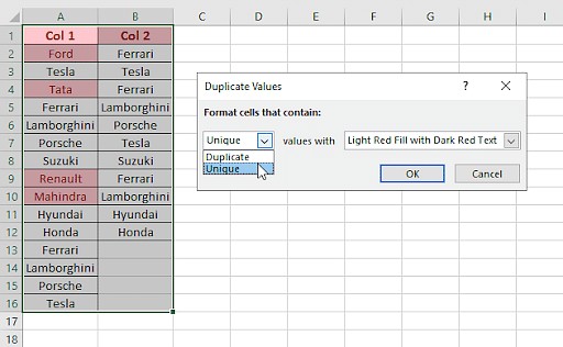
• To highlight matches (duplicates): Ensure “Duplicate” is selected in the dropdown.
• To highlight differences (uniques): Change the dropdown to “Unique.”

Choose a formatting style from the “with” dropdown (e.g., Light Red Fill with Dark Red Text, Yellow Fill, Green Fill, etc.) or customize the formatting by selecting “Custom Format…”. Click “OK” to apply the formatting.

Outcome: Excel will instantly highlight the duplicate or unique values based on your selection, making it easy to visually identify matches and differences between the two columns.

2. Using the Equals Operator (=): Simple Row-by-Row Comparison

The equals operator (=) is the most basic way to compare two columns in Excel on a row-by-row basis. This method is straightforward and quick, especially for simple comparisons.

Steps to Compare Columns Using the Equals Operator:

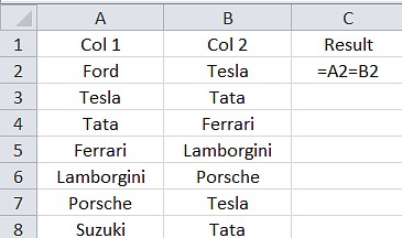
Step 1: Create a Result Column

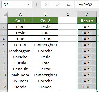
Insert a new column next to the columns you want to compare. This column will display the results of the comparison (TRUE or FALSE). Let’s say you are comparing Column A and Column B, you can create a new column C for the results.

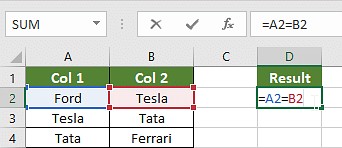
Step 2: Enter the Formula

In the first cell of the result column (e.g., C1), enter the equals formula. To compare cell A1 and B1, the formula would be:

=A1=B1

Press Enter. Excel will display “TRUE” if the values in A1 and B1 are identical, and “FALSE” if they are different.

Step 3: Drag the Formula Down

Click on the fill handle (the small square at the bottom-right corner of cell C1) and drag it down to apply the formula to the rest of the rows in your data.

Step 4: Customize Results with IF Statement (Optional)

For more descriptive results than TRUE/FALSE, you can incorporate the IF formula. For example, to display “Match” for identical values and “Different” for different values, use the following formula in cell C1:

=IF(A1=B1,"Match","Different")

Drag this formula down as before.

Outcome: The result column will clearly indicate whether each corresponding row in the two columns has matching values (“TRUE” or “Match”) or different values (“FALSE” or “Different”).

3. VLOOKUP Function: Finding Matches and Identifying Missing Values

The VLOOKUP function is a powerful tool for searching for a value in a column (lookup column) and returning a corresponding value from the same row in another column. While primarily used for data retrieval, VLOOKUP can also be effectively used to compare columns, especially to identify values in one column that are present or absent in another.

Formula for VLOOKUP:

=VLOOKUP(lookup_value, table_array, col_index_num, [range_lookup])

How to Use VLOOKUP to Compare Columns:

Step 1: Create a Result Column

Similar to the equals operator method, create a new column to display the comparison results.

Step 2: Enter the VLOOKUP Formula

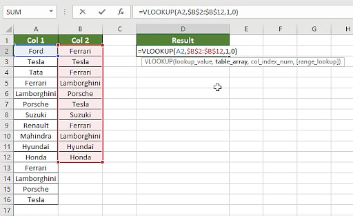
In the first cell of the result column (e.g., C1), enter the VLOOKUP formula. To check if the value in A1 exists in Column B, use the following formula:

=VLOOKUP(A1,B:B,1,FALSE)

• A1 (lookup_value): The value you want to search for (the value in the first cell of Column A).
• B:B (table_array): The column where you want to search for the lookup_value (Column B).
• 1 (col_index_num): We are looking to return a value from the first column of our table_array (which is Column B itself in this case). We just need to know if it exists.
• FALSE ([range_lookup]): Specifies an exact match. We want to find exact matches of A1 in Column B.

Press Enter and drag the formula down to apply it to all rows.

Step 3: Handle Errors (Optional)

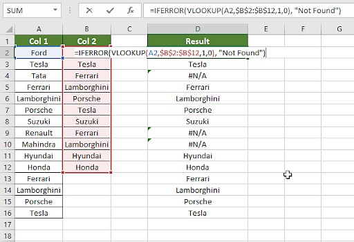
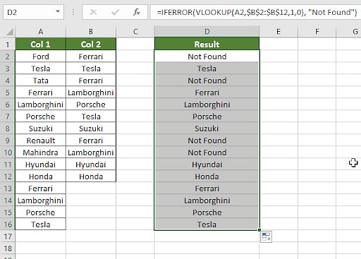
If a value from Column A is not found in Column B, VLOOKUP will return a #N/A error. To display a more user-friendly message instead of the error, use the IFERROR function to wrap the VLOOKUP formula:

=IFERROR(VLOOKUP(A1,B:B,1,FALSE),"Not Found in Column B")

This formula will display “Not Found in Column B” when a value from Column A is not in Column B, and it will display the matching value from Column B if found.

Dealing with Partial Matches and Variations (Wildcards):

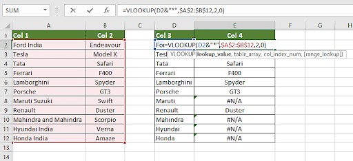
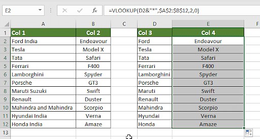
In real-world scenarios, you might encounter slight variations in data, such as “Ford India” in one column and “Ford” in another. Standard VLOOKUP might not recognize these as matches. You can use wildcards within VLOOKUP to handle such cases. For example, to find values in Column A that contain values from Column B, you can modify the formula:

=IFERROR(VLOOKUP("*"&A1&"*",B:B,1,FALSE),"Not Found")

The "*" wildcard character matches any sequence of characters. By adding it before and after A1, we are searching for values in Column B that contain the value from A1. Be cautious when using wildcards, as they can lead to unintended matches if not used carefully.

“` with VLOOKUP to find partial matches.*

Outcome: VLOOKUP is excellent for identifying if values from one column exist in another, and for retrieving corresponding data if matches are found. It’s especially useful when you need to know not just if there’s a match, but also what the matching value is.

4. IF Formula: Customizable Comparison with Textual Results

The IF formula provides a flexible way to compare two columns and return custom text-based results based on whether the values match or not. This is useful when you want to display specific messages like “Match,” “No Match,” “Same,” “Different,” or any other text you define.

Formula for IF:

=IF(logical_test, value_if_true, value_if_false)

Comparing Columns Using the IF Formula:

Step 1: Create a Result Column

Create a new column to display the results of the IF formula.

Step 2: Enter the IF Formula

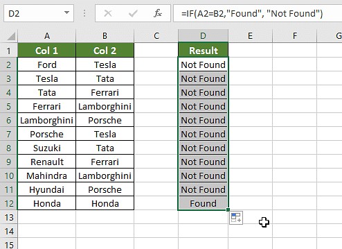
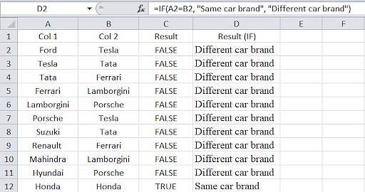
In the first cell of the result column (e.g., C1), enter the IF formula to compare cells in the corresponding rows of the two columns you are comparing (e.g., Column A and Column B). For instance, to display “Same” if values in A1 and B1 are the same, and “Different” otherwise, use:

=IF(A1=B1,"Same","Different")

You can customize the “value_if_true” and “value_if_false” arguments to display any text you need. For example, to compare car brands and display specific messages:

=IF(A1=B1, "Same car brands", "Different car brands")

Press Enter and drag the formula down to apply it to all rows.

Outcome: The result column will display your custom text messages (“Same,” “Different,” “Same car brands,” “Different car brands,” etc.) based on whether the values in the compared columns match or not. The IF formula is highly customizable and allows you to tailor the output to your specific reporting needs.

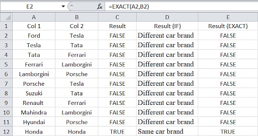
5. EXACT Formula: Case-Sensitive Column Comparison

The EXACT formula in Excel is specifically designed for case-sensitive comparisons. Unlike the equals operator (=) and the IF formula with a simple equality check, EXACT distinguishes between uppercase and lowercase letters. This is crucial when you need to compare text columns where case sensitivity matters (e.g., comparing usernames, codes, or IDs).

Formula for EXACT:

=EXACT(text1, text2)

Using EXACT to Compare Columns:

Step 1: Create a Result Column

Add a new column to hold the results of the EXACT formula.

Step 2: Enter the EXACT Formula

In the first cell of the result column (e.g., C1), enter the EXACT formula to compare corresponding cells from the two columns. For example, to compare A1 and B1:

=EXACT(A1,B1)

Press Enter and drag the formula down.

Outcome: The EXACT formula returns “TRUE” only if the two text strings in the compared cells are exactly the same, including case. If there are any differences in case or characters, it returns “FALSE.” This is particularly useful for scenarios where case sensitivity is important for data accuracy.

Example of Case Sensitivity with EXACT:

If cell A1 contains “Honda” and cell B1 contains “honda,” the formula =EXACT(A1,B1) will return “FALSE” because of the case difference. Only when both cells have the exact same text, including case (e.g., both “Honda”), will EXACT return “TRUE.”

Choosing the Right Method for Your Scenario

Each of these methods has its strengths and is best suited for different scenarios. Here’s a quick guide to help you choose:

Scenario:	Recommended Method(s):	Why?
Quick Visual Overview of Matches/Differences	Conditional Formatting	Fastest visual method, no formulas needed.
Simple Row-by-Row Match/No Match Check	Equals Operator (=)	Very basic and easy to understand, returns TRUE/FALSE.
Custom Text Results for Matches/Differences	IF Formula	Allows for customized text output (e.g., “Match,” “Different”).
Finding Values from One Column in Another (and Identifying Missing Values)	VLOOKUP Function	Powerful for searching and retrieving related data, can identify values not present in the lookup column.
Case-Sensitive Comparison	EXACT Formula	Essential when case sensitivity is critical for accurate comparisons.

Scenarios and Advanced Techniques

Beyond basic comparisons, Excel offers more advanced techniques for specific scenarios.

Scenario 1: Row-by-Row Comparison with Variations

Sometimes, you need to compare rows with slight variations or tolerances.

• Ignoring Extra Spaces: Use the TRIM function within your formulas to remove leading/trailing spaces before comparison: =IF(TRIM(A1)=TRIM(B1),"Match","Different")
• Comparing Numbers within a Range: To check if numbers in two columns are “close enough” (within a certain tolerance), you can use absolute difference and a threshold: =IF(ABS(A1-B1)<0.1,"Close Match","Different") (for a tolerance of 0.1).

Scenario 2: Comparing Multiple Columns for Row Matches

To check if values across multiple columns in the same row are identical, you can use AND and COUNTIF functions.

• Complete Match Across Columns (e.g., Columns A, B, C): =IF(AND(A1=B1, A1=C1), "Complete Match", "")
• Counting Matches Across Columns: =IF(COUNTIF(A1:C1,A1)=3, "Complete Match", "") (where 3 is the number of columns).

Scenario 3: Finding Unique Values (Differences Between Lists)

To find values present in Column A but not in Column B (unique to Column A), use COUNTIF or MATCH with error handling.

• Using COUNTIF: =IF(COUNTIF(B:B,A1)=0, "Unique to Column A", "")
• Using MATCH with IFERROR: =IFERROR(MATCH(A1,B:B,0), "Unique to Column A")

Scenario 4: Comparing Lists and Pulling Matching Data

For comparing lists and retrieving matching data, VLOOKUP and INDEX-MATCH are excellent.

• VLOOKUP (as demonstrated earlier): =VLOOKUP(D1,A:B,2,FALSE) (looks up values from Column D in Column A and returns corresponding values from Column B).
• INDEX-MATCH (more flexible than VLOOKUP): =INDEX(B:B, MATCH(D1,A:A,0)) (achieves the same as VLOOKUP but with more flexibility).
• XLOOKUP (modern alternative to VLOOKUP and INDEX-MATCH, available in newer Excel versions): =XLOOKUP(D1,A:A,B:B) (simplifies the lookup process).

Scenario 5: Highlighting Row Matches and Differences Across Multiple Columns

Conditional formatting can be extended to highlight entire rows based on matches or differences across multiple columns.

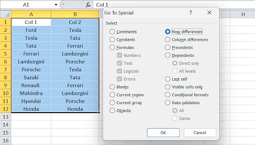
• Highlight Rows with Identical Values in Columns A, B, C: Select columns A, B, and C. Go to Conditional Formatting > New Rule > Use a formula to determine which cells to format. Enter the formula: =AND($A1=$B1, $A1=$C1). Choose formatting and apply.
• Highlight Row Differences Using “Go To Special”: Select the data range. Press Ctrl+G (Go To Special) > Row Differences > OK. This will select cells that are different from the corresponding cell in the same row, which you can then format.

Frequently Asked Questions (FAQs)

1. What is the quickest way to compare two columns in Excel?

Conditional Formatting is the quickest way for a visual comparison. For formula-based comparison, the Equals Operator (=) is the simplest and fastest to set up.

2. Can I compare two columns in Excel using the INDEX-MATCH function?

Yes, INDEX-MATCH is a powerful and flexible way to compare columns, especially when you need to retrieve corresponding data or handle more complex lookup scenarios.

3. How do I compare multiple columns in Excel for duplicates?

Use Conditional Formatting and choose “Duplicate Values.” Select all the columns you want to compare. Excel will highlight values that are duplicated across the selected columns.

4. How can I compare two lists in Excel and find matches?

You can use VLOOKUP, INDEX-MATCH, or XLOOKUP to compare two lists and find matching values. Conditional Formatting (Duplicate Values) can also visually highlight matches between two lists.

5. How do I compare two columns in Excel and highlight the differences?

Use Conditional Formatting and choose “Unique Values” to highlight values that are different between two columns. Alternatively, use the Equals Operator (=) or IF formula to identify differences and then use Conditional Formatting to highlight the rows where the result is “FALSE” or “Different.”

Next Steps: Beyond Column Comparison

Mastering column comparison in Excel is a crucial step in data analysis. To further enhance your Excel skills and data analysis capabilities, consider exploring:

• Pivot Tables and Pivot Charts: For summarizing and visualizing data from your compared columns. Pivot tables are excellent for creating dynamic summaries and performing further analysis on matched and unmatched data.
• Excel Functions for Data Cleaning: Learn more functions like TRIM, CLEAN, SUBSTITUTE, and TEXT to prepare your data for accurate comparisons.
• Power Query (Get & Transform Data): For more advanced data manipulation, cleaning, and comparison tasks, especially when dealing with large datasets or data from multiple sources. Power Query offers powerful tools for merging, appending, and transforming data before analysis.

By mastering these techniques, you’ll be well-equipped to efficiently analyze and compare data in Excel, making you a more proficient data professional.