Excel Formula to Compare Two Columns for Matches: A Comprehensive Guide

In the realm of data analysis, especially when using tools like Excel, the need to compare columns for matching data arises frequently. Whether you are reconciling datasets, identifying duplicates, or simply ensuring data consistency, manual comparison can be time-consuming and error-prone, particularly with large datasets. Fortunately, Excel offers a variety of powerful formulas to automate this process, saving you valuable time and enhancing accuracy.

This guide will explore several effective Excel formulas to compare two columns for matches, catering to different scenarios and complexity levels. We will delve into each method with step-by-step instructions and practical examples, empowering you to efficiently analyze your data and extract meaningful insights.

Understanding Column Comparison in Excel

Comparing columns in Excel involves checking corresponding cells across two columns to determine if their values are identical or if there are any discrepancies. This comparison can be for exact matches, partial matches, or even based on specific criteria. The outcome of such comparisons can be used for various purposes, such as highlighting matching entries, extracting unique values, or triggering actions based on the comparison result.

Let’s dive into the methods you can use to achieve this effectively.

Methods to Compare Two Columns for Matches in Excel

Excel provides several built-in features and formulas to compare columns efficiently. Here are some of the most commonly used and effective methods:

1. Conditional Formatting for Quick Visual Comparison

Conditional formatting is a simple yet powerful feature in Excel that allows you to visually highlight cells based on specific criteria. It’s an excellent method for a quick overview and identifying matches or differences between two columns without using formulas directly.

Steps to use Conditional Formatting:

1. Select the Columns: Begin by selecting the two columns you wish to compare. You can select entire columns by clicking on the column headers (e.g., ‘A’ and ‘B’) or select specific ranges of cells.

2. Access Conditional Formatting: Navigate to the “Home” tab on the Excel ribbon. In the “Styles” group, click on “Conditional Formatting.”

3. Highlight Duplicate or Unique Values: From the dropdown menu, choose “Highlight Cells Rules,” and then select either “Duplicate Values” or “Unique Values” depending on what you want to identify.

4. Choose Formatting Style: A dialog box will appear where you can select the formatting style to be applied to the duplicate or unique values. You can choose from predefined styles or customize your own. Click “OK” to apply the formatting.

Conditional Formatting is ideal for quickly spotting matches or unique entries visually, but it doesn’t provide a text-based output like formulas do. For more detailed analysis and text-based results, formulas are necessary.

2. Using the Equals Operator (=) for Direct Comparison

The equals operator (=) is the most basic formula for comparing two cells in Excel. It returns TRUE if the cell values are identical and FALSE otherwise. This method is straightforward and perfect for simple, row-by-row comparisons.

Steps to use the Equals Operator:

1. Create a Result Column: Insert a new column next to the columns you are comparing. This column will display the results of the comparison. For example, if you are comparing columns A and B, you might create a result column in C.

2. Enter the Formula: In the first cell of your result column (e.g., C2), enter the formula =A2=B2. This formula compares the value in cell A2 with the value in cell B2.

3. Apply to Entire Column: Drag the fill handle (the small square at the bottom-right corner of the selected cell) down to apply the formula to all rows in your dataset. Excel will automatically adjust the cell references for each row.

Customizing Results with the IF Function:

You can enhance the output by using the IF function to display custom messages instead of TRUE and FALSE. For example, to display “Match” for true comparisons and “Mismatch” for false ones, use the formula: =IF(A2=B2, "Match", "Mismatch").

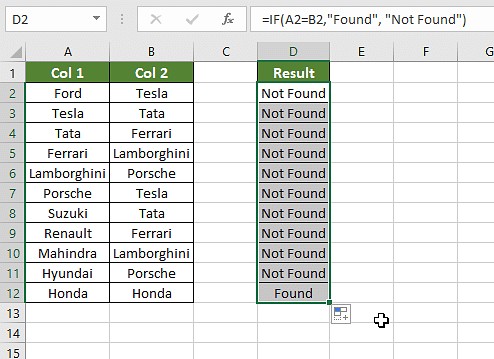![Using IF clause to customize results of equals operator in Excel](http://compare.edu.vn/wp-content/uploads/2025/02/comparecolumnsinexcel9.jpg){width=494 height=359}
*Alt Text: Column C showing customized results "Match" and "Mismatch" using the IF function in conjunction with the equals operator.*

The equals operator is simple and effective for basic comparisons, but it lacks flexibility for more complex scenarios like partial matches or comparisons across datasets.

3. Leveraging the VLOOKUP Function for List Comparison

The VLOOKUP function is a powerful tool for comparing data in one column against another and retrieving corresponding information. It’s particularly useful when you want to check if values from one column exist in another and potentially pull related data.

Formula Syntax:

=VLOOKUP(lookup_value, table_array, col_index_num, [range_lookup])

• lookup_value: The value you want to search for (e.g., a cell from the first column).
• table_array: The range of cells in the second column where you want to search for the lookup_value.
• col_index_num: The column number within the table_array from which to return a value (typically 1 when just checking for a match).
• [range_lookup]: FALSE for exact match (recommended for column comparison).

Steps to use VLOOKUP for column comparison:

1. Create a Result Column: Similar to the equals operator method, add a new column for the results.

2. Enter the VLOOKUP Formula: In the first cell of the result column, enter the VLOOKUP formula. For example, to check if values in column A are present in column B, in cell C2, enter: =VLOOKUP(A2, B:B, 1, FALSE). Here, A2 is the lookup_value, B:B is the table_array (entire column B), 1 is the col_index_num (we are interested if the value from column A is found in column B), and FALSE ensures an exact match.

3. Apply to Entire Column: Drag the fill handle down to apply the formula to all rows.

Handling Errors with IFERROR:

VLOOKUP returns #N/A errors when a match is not found. To display a more user-friendly message, you can use the IFERROR function to replace errors with custom text like “Not Found”. The modified formula would be: =IFERROR(VLOOKUP(A2, B:B, 1, FALSE), "Not Found").

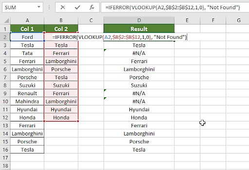![Using IFERROR with VLOOKUP to handle errors and display custom message](http://compare.edu.vn/wp-content/uploads/2025/02/comparecolumnsinexcel12.jpg){width=512 height=350}
*Alt Text: Formula bar showing the combined formula '=IFERROR(VLOOKUP(A2, B:B, 1, FALSE), "Not Found")' to manage #N/A errors from VLOOKUP.*

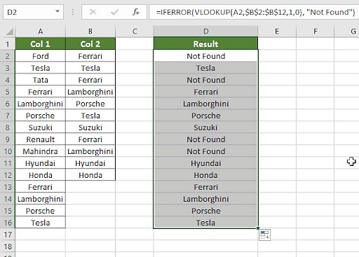![Error-free results with IFERROR and VLOOKUP displaying "Not Found"](http://compare.edu.vn/wp-content/uploads/2025/02/comparecolumnsinexcel13.jpg){width=512 height=367}
*Alt Text: Column C showing results with values from column B for matches and "Not Found" for mismatches, replacing #N/A errors with a user-friendly message.*

Handling Partial Matches with Wildcards:

In scenarios where you need to find partial matches (e.g., “Ford India” matching “Ford”), you can use wildcards in conjunction with VLOOKUP. For instance, to find values in column A that partially match values in column C, you might use a formula like: =IFERROR(VLOOKUP(A2&"*", C:C, 1, FALSE), "Not Found"). The &"*" appends a wildcard character to the lookup_value, allowing for partial matches. Be cautious when using wildcards as they can lead to unintended matches.

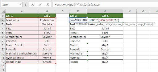![Using wildcard with VLOOKUP for partial matches in column comparison](http://compare.edu.vn/wp-content/uploads/2025/02/comparecolumnsinexcel15.jpg){width=512 height=234}
*Alt Text: Formula bar showing '=IFERROR(VLOOKUP(A2&"*", C:C, 1, FALSE), "Not Found")' using a wildcard to find partial matches.*

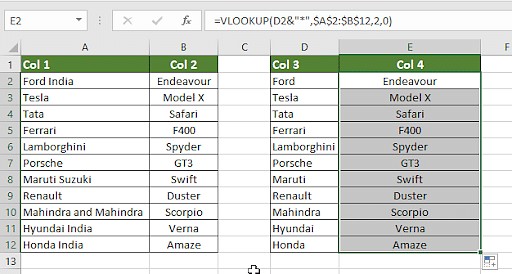![Results of VLOOKUP with wildcard showing matches for partial values](http://compare.edu.vn/wp-content/uploads/2025/02/comparecolumnsinexcel16.jpg){width=512 height=274}
*Alt Text: Column C displaying results where partial matches are found using the wildcard in the VLOOKUP formula, effectively comparing values with slight variations.*

VLOOKUP is versatile for list comparisons and can be adapted for various matching scenarios, including handling errors and partial matches.

4. Utilizing the IF Formula for Conditional Outcomes

The IF formula provides a way to perform logical comparisons and return different results based on whether the condition is true or false. It’s highly flexible for creating custom outputs based on column comparisons.

Formula Syntax:

=IF(logical_test, value_if_true, value_if_false)

• logical_test: The condition you want to evaluate (e.g., A2=B2).
• value_if_true: The value to return if the logical_test is true.
• value_if_false: The value to return if the logical_test is false.

Example using IF to compare car brands:

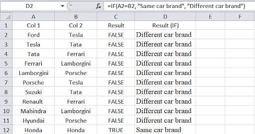
Suppose you want to compare car brands in column A and column B and display “Same car brands” if they match and “Different car brands” if they don’t. You would use the following formula in column D: =IF(A2=B2, "Same car brands", "Different car brands").

![Using IF Formula to compare car brands and display custom messages](http://compare.edu.vn/wp-content/uploads/2025/02/ifformula1.jpg){width=512 height=270}
*Alt Text: Column D showing results "Same car brands" and "Different car brands" based on the IF formula comparing columns A and B for matching car brands.*

The IF formula is excellent for creating conditional outputs based on column comparisons, allowing for customized messages and actions based on match results.

5. Employing the EXACT Formula for Case-Sensitive Comparisons

The EXACT formula in Excel is designed for case-sensitive comparisons. Unlike the equals operator (=), which is case-insensitive, EXACT distinguishes between uppercase and lowercase characters.

Formula Syntax:

=EXACT(text1, text2)

• text1: The first text string to compare.
• text2: The second text string to compare.

EXACT returns TRUE if text1 and text2 are exactly the same, including case, and FALSE otherwise.

Example of Case-Sensitive Comparison:

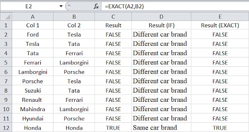
To compare values in column A and column B case-sensitively, use the formula =EXACT(A2, B2). This will return TRUE only if the content and case of cell A2 and B2 are identical.

![Using EXACT formula for case-sensitive comparison in Excel](http://compare.edu.vn/wp-content/uploads/2025/02/exactformula2.jpg){width=512 height=271}
*Alt Text: Column C showing TRUE and FALSE results from the EXACT formula, highlighting its case-sensitive nature in comparing column A and B values.*

It’s important to remember that EXACT is case-sensitive. For example, "Honda" and "honda" would be considered different by the EXACT formula, resulting in a FALSE output. If case sensitivity is crucial for your comparison, EXACT is the ideal formula.

Choosing the Right Method for Your Scenario

The best method for comparing two columns in Excel depends on your specific needs and the complexity of your data. Here’s a guide to help you choose:

Scenario 1: Row-by-Row Comparison for Simple Matches

For basic row-by-row comparisons where you need to know if values in two columns are the same in each row, the Equals Operator (=) or the IF formula are the simplest and most efficient.

• Equals Operator: =A2=B2 (Returns TRUE or FALSE)

• IF Formula: =IF(A2=B2, "Match", "Mismatch") (Returns custom text)

• Case-Sensitive IF with EXACT: =IF(EXACT(A2, B2), "Match", "Mismatch") (For case-sensitive matching)

Scenario 2: Comparing Multiple Columns for Row Matches

When you need to compare more than two columns in each row to find complete matches across all columns or identify rows with any matching values, you can use combinations of IF, AND, OR, and COUNTIF functions.

• Complete Match Across Columns (e.g., A, B, C): =IF(AND(A2=B2, A2=C2), "Complete Match", "")
• Complete Match Across a Range (e.g., A to E, assuming 5 columns): =IF(COUNTIF($A2:$E2, $A2)=5, "Complete Match", "") (Adjust ‘5’ to the number of columns)
• Any Match in Row (e.g., A, B, C): =IF(OR(A2=B2, B2=C2, A2=C2), "Match", "")

Scenario 3: Finding Matches and Differences Between Two Lists

To compare two lists (columns) and identify unique values in one list that are not present in the other, or vice versa, VLOOKUP or COUNTIF are effective.

• Values in Column A Not in Column B (using COUNTIF): =IF(COUNTIF(B:B, A2)=0, "Not in B", "")
• Values in Column A Not in Column B (using ISERROR and MATCH): =IF(ISERROR(MATCH(A2, B:B, 0)), "Not in B", "")
• Matches and Differences (using COUNTIF): =IF(COUNTIF(B:B, A2)=0, "Not in B", "Present in B")

Scenario 4: Comparing Lists and Extracting Matching Data

If you need to compare two lists and, when a match is found, pull corresponding data from the second list, VLOOKUP, INDEX MATCH, or XLOOKUP are suitable.

• VLOOKUP (to get value from column B if A2 is in column D): =VLOOKUP(D2, $A$2:$B$6, 2, FALSE) (Adjust ranges as needed)
• INDEX MATCH (more flexible lookup): =INDEX($B$2:$B$6, MATCH(D2, $A$2:$A$6, 0))
• XLOOKUP (modern and versatile): =XLOOKUP(D2, $A$2:$A$6, $B$2:$B$6)

Scenario 5: Highlighting Row Matches and Differences Visually

For visually highlighting entire rows based on matches or differences across columns, Conditional Formatting with formulas is the way to go.

• Highlight Rows with Identical Values in Columns A, B, and C:

  1. Select the range of data.
  2. Go to Conditional Formatting > New Rule > Use a formula to determine which cells to format.
  3. Enter the formula: =AND($A2=$B2, $A2=$C2) (for complete row match) or =COUNTIF($A2:$C2, $A2)=3 (adjust ‘3’ for column count).
  4. Choose your formatting style and apply.

• Highlight Row Differences Using “Go To Special”:

  1. Select the data range.
  2. Press Ctrl + G (or F5) to open “Go To” dialog, click “Special.”
  3. Choose “Row Differences” and click “OK.”
  4. Excel will select cells with differences in each row, which you can then format.

Frequently Asked Questions (FAQs)

1. What is the quickest way to compare two columns in Excel?

The quickest way to visually compare two columns is using Conditional Formatting to highlight duplicate or unique values. For formula-based comparison, the equals operator (=) is the fastest for simple row-by-row checks.

2. Can I compare two columns using INDEX-MATCH?

Yes, INDEX-MATCH is a powerful and flexible method for comparing columns, especially when you need to retrieve corresponding data based on matches. It’s often preferred over VLOOKUP for its flexibility.

3. How do I compare multiple columns at once for matches?

You can compare multiple columns using Conditional Formatting by selecting all columns and highlighting duplicates or uniques. For formula-based comparison, use AND, OR, or COUNTIF functions as demonstrated in Scenario 2.

4. How can I compare two lists in Excel and find the matches?

Use VLOOKUP, MATCH, or COUNTIF to compare two lists and find matches. VLOOKUP and MATCH are particularly useful for checking if values from one list exist in another, while COUNTIF can count the occurrences of matches.

5. How do I compare two columns and highlight duplicates?

To highlight duplicates in two columns:

1. Select both columns.
2. Go to Home > Conditional Formatting > Highlight Cells Rules > Duplicate Values.
3. Choose your desired formatting and click “OK.”

This will highlight all duplicate values found in the selected columns.

Next Steps in Excel Data Analysis

Mastering column comparison techniques is a fundamental step in Excel data analysis. To further enhance your skills, consider exploring Pivot Tables and Charts in Excel for summarizing and visualizing data. These tools can transform raw data into insightful reports and interactive dashboards, building upon your ability to effectively compare and analyze data within Excel.

Continue your journey to become a proficient data analyst by exploring advanced Excel functions and data analysis techniques. With the right skills, you can unlock the full potential of Excel for data-driven decision-making.