Excel Comparing 2 Columns: Comprehensive Guide For Data Analysis

Excel Comparing 2 Columns is crucial for data analysis. COMPARE.EDU.VN offers comprehensive solutions for effectively comparing data in Excel, identifying matches and differences between columns, and making informed decisions. Learn techniques for data comparison, duplicate detection, and unique value identification with our guides.

1. Understanding the Importance of Excel Comparing 2 Columns

Comparing two columns in Excel is a fundamental skill for anyone working with data. Whether you’re a student comparing research data, a business professional analyzing sales figures, or an analyst identifying discrepancies, understanding how to effectively compare columns in Excel can save you time and improve your accuracy. This guide, brought to you by COMPARE.EDU.VN, will walk you through various methods, from simple formulas to advanced techniques, to help you master this essential skill. Leverage Excel comparison techniques for accurate data analysis, efficient data matching, and effective difference identification.

2. Basic Techniques for Excel Comparing 2 Columns Row-by-Row

When dealing with data, one of the most common tasks is comparing two columns on a row-by-row basis. Microsoft Excel provides several ways to accomplish this, with the IF function being a primary tool. Here are some examples of how you can use the IF function to compare columns effectively.

2.1. Identifying Matches and Differences in the Same Row

The IF function in Excel is perfect for comparing values in the same row across two columns.

2.1.1. Formula for Finding Matches

To find cells with identical content (e.g., A2 and B2), use the following formula:

=IF(A2=B2,"Match","")

This formula returns “Match” if the values in cells A2 and B2 are the same, and an empty string if they are different.

2.1.2. Formula for Finding Differences

To find cells with different values, replace the equals sign (=) with the not equals sign (<>):

=IF(A2<>B2,"No match","")

This formula returns “No match” if the values in cells A2 and B2 are different, and an empty string if they are the same.

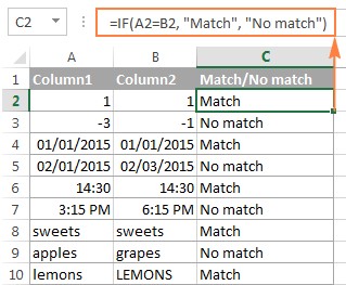
2.1.3. Combining Matches and Differences

You can combine the formulas to identify both matches and differences in one go:

=IF(A2=B2,"Match","No match")

Or:

=IF(A2<>B2,"No match","Match")

These formulas return “Match” if the values are the same and “No match” if they are different.

These formulas work well with numbers, dates, times, and text strings. Using formulas for Excel data validation ensures accuracy, helps in data reconciliation, and supports effective data matching strategies.

2.2. Performing Case-Sensitive Comparisons

The above formulas ignore case when comparing text values. To perform a case-sensitive comparison, use the EXACT function.

2.2.1. Formula for Case-Sensitive Matches

To find cells with the same content, including case, use:

=IF(EXACT(A2, B2), "Match", "")

This formula returns “Match” only if the values in A2 and B2 are identical, including case.

2.2.2. Formula for Case-Sensitive Differences

To find case-sensitive differences, modify the formula:

=IF(EXACT(A2, B2), "Match", "Unique")

This formula returns “Match” if the values are identical and “Unique” if they are different, considering case.

Case-sensitive comparison enhances data integrity, provides precise matching, and strengthens data accuracy in Excel.

3. Advanced Techniques: Excel Comparing Multiple Columns

Excel also allows you to compare more than two columns at once. Here are some methods to do this effectively.

3.1. Finding Matches in All Cells Within the Same Row

When you need to compare three or more columns and find rows where all cells have the same values, you can use an IF formula with an AND statement or the COUNTIF function.

3.1.1. Using IF and AND

For tables with a few columns, an IF formula with an AND statement works well:

=IF(AND(A2=B2, A2=C2), "Full match", "")

This formula returns “Full match” only if the values in A2, B2, and C2 are identical.

3.1.2. Using COUNTIF

For tables with many columns, COUNTIF provides a more elegant solution:

=IF(COUNTIF($A2:$E2, $A2)=5, "Full match", "")

Here, 5 represents the number of columns being compared (A to E).

Using Excel formulas for duplicate checking ensures data consistency, improves data quality, and reduces errors in large datasets.

3.2. Finding Matches in Any Two Cells in the Same Row

If you need to identify rows where any two or more cells have the same values, you can use an IF formula with an OR statement or combine multiple COUNTIF functions.

3.2.1. Using IF and OR

For a few columns, use an IF formula with an OR statement:

=IF(OR(A2=B2, B2=C2, A2=C2), "Match", "")

This formula returns “Match” if any two cells (A2 and B2, B2 and C2, or A2 and C2) have the same values.

3.2.2. Using Multiple COUNTIF Functions

For many columns, combine COUNTIF functions:

=IF(COUNTIF(B2:D2,A2)+COUNTIF(C2:D2,B2)+(C2=D2)=0,"Unique","Match")

This formula returns “Match” if any values are repeated and “Unique” if all values are different. Employing Excel’s data comparison tools streamlines data analysis, provides actionable insights, and improves decision-making processes.

4. Comparing Two Columns for Matches and Differences

Sometimes, you need to compare two columns to find values that are present in one column but not in the other. You can achieve this using the COUNTIF function within an IF formula.

4.1. Identifying Values in Column A Not Present in Column B

To find values in column A that are not in column B, use:

=IF(COUNTIF($B:$B, $A2)=0, "No match in B", "")

This formula checks if the value in A2 exists in column B. If it doesn’t, it returns “No match in B”.

4.2. Using ISERROR and MATCH Functions

Alternatively, you can use ISERROR and MATCH:

=IF(ISERROR(MATCH($A2,$B$2:$B$10,0)),"No match in B","")

This formula attempts to find the value in A2 within the range B2:B10. If it fails, it returns “No match in B”.

4.3. Using Array Formulas

An array formula can also achieve this:

=IF(SUM(--($B$2:$B$10=$A2))=0, " No match in B", "")

Remember to press Ctrl + Shift + Enter when entering array formulas.

4.4. Identifying Both Matches and Differences

To identify both matches and differences, modify the COUNTIF formula:

=IF(COUNTIF($B:$B, $A2)=0, "No match in B", "Match in B")

This formula returns “No match in B” if the value is not found and “Match in B” if it is. Identifying data differences helps in data cleansing, ensures data compliance, and enhances data governance.

5. Pulling Matching Data from Two Lists

Often, you may want to not only compare two columns but also extract matching entries from a lookup table. Excel offers several functions for this, including VLOOKUP, INDEX MATCH, and XLOOKUP.

5.1. Using VLOOKUP

VLOOKUP is a classic function for pulling matching data:

=VLOOKUP(D2, $A$2:$B$6, 2, FALSE)

This formula compares the value in D2 against column A and pulls the corresponding value from column B.

5.2. Using INDEX MATCH

INDEX MATCH is a more versatile alternative:

=INDEX($B$2:$B$6, MATCH($D2, $A$2:$A$6, 0))

This formula does the same as VLOOKUP but is more flexible and powerful.

5.3. Using XLOOKUP (Excel 2021 and Excel 365)

XLOOKUP is the newest and most advanced option:

=XLOOKUP(D2, $A$2:$A$6, $B$2:$B$6)

XLOOKUP simplifies the process and offers better error handling.

These formulas facilitate data integration, streamline reporting processes, and improve data lookup efficiency.

6. Highlighting Matches and Differences in Excel

Highlighting matches and differences can visually enhance your data comparison. Excel’s Conditional Formatting feature is ideal for this.

6.1. Highlighting Matches and Differences in Each Row

6.1.1. Highlighting Matches

To highlight cells in column A that have identical entries in column B:

Select the cells in column A.
Go to Conditional Formatting > New Rule > Use a formula to determine which cells to format.
Enter the formula: =$B2=$A2

6.1.2. Highlighting Differences

To highlight cells with different values:

Select the cells in column A.
Go to Conditional Formatting > New Rule > Use a formula to determine which cells to format.
Enter the formula: =$B2<>$A2

6.2. Highlighting Unique Entries in Each List

To highlight items that are unique to each list:

6.2.1. Unique Values in List 1 (Column A)

Select the cells in column A.
Go to Conditional Formatting > New Rule > Use a formula to determine which cells to format.
Enter the formula: =COUNTIF($C$2:$C$5, $A2)=0

6.2.2. Unique Values in List 2 (Column C)

Select the cells in column C.
Go to Conditional Formatting > New Rule > Use a formula to determine which cells to format.
Enter the formula: =COUNTIF($A$2:$A$6, $C2)=0

6.3. Highlighting Matches (Duplicates) Between Two Columns

To highlight duplicate values:

6.3.1. Matches in List 1 (Column A)

Select the cells in column A.
Go to Conditional Formatting > New Rule > Use a formula to determine which cells to format.
Enter the formula: =COUNTIF($C$2:$C$5, $A2)>0

6.3.2. Matches in List 2 (Column C)

Select the cells in column C.
Go to Conditional Formatting > New Rule > Use a formula to determine which cells to format.
Enter the formula: =COUNTIF($A$2:$A$6, $C2)>0

Conditional formatting enhances data visibility, helps in data validation, and improves data analysis workflows.

7. Highlighting Row Differences and Matches in Multiple Columns

When you’re comparing values across multiple columns, highlighting matches and differences can be very useful.

7.1. Highlighting Rows with Identical Values in All Columns

To highlight rows that have the same values in all columns:

Select the data range.
Go to Conditional Formatting > New Rule > Use a formula to determine which cells to format.
Enter the formula: =AND($A2=$B2, $A2=$C2)

Alternatively, use:

=COUNTIF($A2:$C2, $A2)=3

Here, 3 represents the number of columns being compared.

7.2. Highlighting Row Differences in Multiple Columns

To quickly highlight cells with different values in each row:

Select the range of cells to compare.
Go to the Home tab > Editing group > Find & Select > Go To Special.
Select Row differences and click OK.
Choose a fill color to highlight the differences.

This feature helps in quickly identifying discrepancies, facilitates data auditing, and ensures data accuracy in complex datasets.

8. Comparing Two Cells in Excel

Comparing two cells is a simplified version of comparing two columns. You can use the same formulas as above, but without copying them down to other cells.

8.1. For Matches

=IF(A1=C1, "Match", "")

8.2. For Differences

=IF(A1<>C1, "Difference", "")

This method is straightforward, provides instant results, and helps in quick data verification.

9. Simplifying Column Comparison with COMPARE.EDU.VN

At COMPARE.EDU.VN, we understand the challenges of comparing data and making informed decisions. Our platform is designed to provide you with comprehensive, objective comparisons across various products, services, and ideas.

9.1. Why Choose COMPARE.EDU.VN?

Objective Comparisons: We offer unbiased comparisons based on thorough research and analysis.
Detailed Information: Our comparisons include features, specifications, pricing, and user reviews.
User-Friendly Interface: Easily navigate and find the comparisons you need.
Time-Saving: Get all the information you need in one place, saving you hours of research.
Informed Decisions: Make confident decisions with clear, concise comparisons.

9.2. How COMPARE.EDU.VN Helps You

Comprehensive Analysis: We delve into every aspect of the items being compared, ensuring you have a complete picture.
Pros and Cons: We present the advantages and disadvantages of each option, helping you weigh the trade-offs.
Side-by-Side Comparisons: Our tables and lists make it easy to see the differences and similarities at a glance.
User Reviews: Benefit from the experiences of others, adding a layer of real-world insight to your decision-making process.

10. FAQs About Excel Comparing 2 Columns

How do I compare two columns in Excel for exact matches?
- Use the EXACT function within an IF statement: =IF(EXACT(A2, B2), "Match", "No Match").
Can I compare two columns for partial matches?
- Yes, use the SEARCH or FIND function. For example: =IF(ISNUMBER(SEARCH(A2, B2)), "Partial Match", "No Match").
How can I ignore case sensitivity when comparing two columns?
- Use the UPPER or LOWER functions to convert the text to the same case before comparing. For example: =IF(UPPER(A2)=UPPER(B2), "Match", "No Match").
Is it possible to compare two columns and return a value from a third column if there’s a match?
- Yes, use the VLOOKUP, INDEX/MATCH, or XLOOKUP functions.
How do I highlight duplicate values across two columns?
- Use conditional formatting with the COUNTIF function.
What is the best way to compare two large lists in Excel?
- Use array formulas or the COUNTIF function. For very large lists, consider using Excel’s Power Query for better performance.
How can I compare two columns and identify unique values in each column?
- Use the COUNTIF function in conditional formatting rules or in a separate column with an IF statement.
Can I compare two columns with dates?
- Yes, use the same comparison operators (=, <>, <, >) as with numbers or text. Ensure the dates are formatted correctly.
How do I compare two columns and return the number of matches?
- Use the SUMPRODUCT function with a comparison. For example: =SUMPRODUCT(--(A1:A10=B1:B10)).
What are some common errors when comparing two columns in Excel and how can I avoid them?
- Common errors include incorrect cell references, forgetting to use absolute references ($), and not handling case sensitivity or data type differences. Double-check your formulas and use appropriate functions to handle these issues.

11. Ready to Make Smarter Choices?

Comparing data in Excel doesn’t have to be a daunting task. By following the methods outlined in this guide, you can efficiently analyze your data and make informed decisions. For more comprehensive comparisons and to simplify your decision-making process, visit COMPARE.EDU.VN today.

11.1. Take the Next Step

Visit COMPARE.EDU.VN to explore our detailed comparisons and find the perfect solution for your needs. Our platform is designed to provide you with the information you need to make confident, informed decisions.

Contact Us:

Address: 333 Comparison Plaza, Choice City, CA 90210, United States
WhatsApp: +1 (626) 555-9090
Website: COMPARE.EDU.VN

Start comparing now and make smarter choices with compare.edu.vn Data comparisons using conditional formatting offer visual insights, provide actionable data, and ensure consistent data interpretation.