
Comparing values in two columns in Excel is a common task in data analysis. Whether you’re auditing data, merging lists, or identifying discrepancies, manually comparing columns can be time-consuming and prone to error, especially with large datasets. Fortunately, Excel offers several efficient methods to compare values in two columns and highlight matches or differences within seconds. This guide will explore various techniques, from simple conditional formatting to powerful formulas, to help you master column comparison in Excel and boost your data analysis efficiency.
Understanding Column Comparison in Excel
At its core, comparing columns in Excel involves examining corresponding cells in two columns to determine if their values match or differ. This comparison can be used to identify:
- Matches: Rows where values in the specified columns are identical.
- Differences: Rows where values in the specified columns are not the same.
- Unique Values: Values present in one column but not in another.
- Duplicates: Values that appear in both columns.
Excel provides a range of tools and functions to automate this process, allowing you to quickly analyze and visualize the comparison results.
Effective Methods to Compare Two Columns in Excel
Here are several methods you can use to compare values in two columns in Excel, ranging from user-friendly features to formula-based approaches:
1. Conditional Formatting: Visually Highlight Matches and Differences
Conditional formatting is a quick and visual way to compare columns and highlight matching or unique values directly within your spreadsheet.
Steps:
-
Select the Columns: Choose the two columns you want to compare. You can select entire columns by clicking on the column letters (e.g., ‘A’ and ‘B’) or select specific ranges of cells.
-
Access Conditional Formatting: Go to the “Home” tab on the Excel ribbon. In the “Styles” group, click on “Conditional Formatting.”
-
Highlight Duplicate or Unique Values: From the dropdown menu, select “Highlight Cells Rules,” and then choose either “Duplicate Values” or “Unique Values,” depending on what you want to highlight.
-
Customize Formatting: A dialog box will appear. Choose whether you want to highlight “Duplicate” or “Unique” values. Select the formatting style you prefer (e.g., fill color, font color) from the dropdown, or customize the format further. Click “OK.”
Excel will instantly highlight the cells based on your chosen criteria (duplicate or unique values) across the selected columns, providing a visual comparison.
2. Equals Operator (=): Simple Row-by-Row Comparison
The equals operator (=) is the most basic way to compare cells in Excel. You can use it to perform a row-by-row comparison and return TRUE for matches and FALSE for differences.
Steps:
-
Insert a Result Column: Create a new column next to the columns you are comparing (e.g., Column C if you are comparing Column A and Column B). This column will display the comparison results.
-
Enter the Formula: In the first cell of the result column (e.g., C2), enter the formula
=A2=B2. This formula compares the value in cell A2 with the value in cell B2. -
Apply the Formula: Drag the fill handle (the small square at the bottom-right corner of the selected cell) down to apply the formula to the rest of the rows in your data.
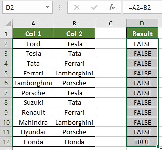
Excel will display “TRUE” in the result column for rows where the values in Column A and Column B are identical and “FALSE” where they differ.
{width=330 height=306}
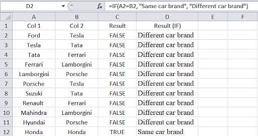
*The result of the equals operator comparison, showing TRUE for matches and FALSE for differences.*Customizing Results with IF Formula:
You can enhance the output by using the IF formula to display custom messages instead of TRUE/FALSE. For example, use the formula =IF(A2=B2, "Match", "Different") to display “Match” for identical values and “Different” for dissimilar values.
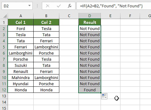{width=494 height=359}
*Customizing the comparison result using the IF formula to display "Match" and "Different" instead of TRUE/FALSE.*3. VLOOKUP Function: Finding Matches and Identifying Missing Values
The VLOOKUP function is useful for comparing columns when you want to check if values from one column exist in another column and potentially retrieve corresponding data.
Formula:
=VLOOKUP(lookup_value, table_array, col_index_num, [range_lookup])
How to use VLOOKUP for column comparison:
-
Set up the Formula: In a result column, enter the VLOOKUP formula. For instance, to check if values in Column A exist in Column B, in cell C2, enter
=VLOOKUP(A2, B:B, 1, FALSE).A2: The lookup value (the value from Column A you are checking).B:B: The table array (Column B, where you are looking for matches).1: The column index number (since we are looking up in a single column, it’s 1).FALSE: For an exact match.
-
Apply and Interpret Results: Drag the formula down.
- If VLOOKUP finds a match, it will return the matching value from Column B.
- If VLOOKUP does not find a match, it will return a #N/A error.
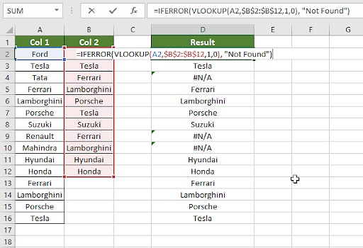
Handling Errors with IFERROR:
To replace the #N/A errors with more user-friendly messages, use the IFERROR function. Wrap your VLOOKUP formula within IFERROR like this: =IFERROR(VLOOKUP(A2, B:B, 1, FALSE), "Not Found in Column B").
{width=512 height=350}
*Implementing IFERROR to replace #N/A errors with a custom "Not Found" message.*Now, instead of errors, you will see “Not Found in Column B” for values from Column A that are not present in Column B.
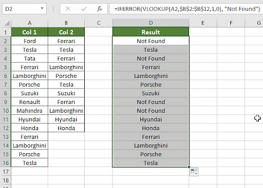{width=512 height=367}
*Error-free VLOOKUP results, displaying "Not Found in Column B" for unmatched values.*Handling Partial Matches with Wildcards:
In cases where you need to compare columns with slight variations in text (e.g., “Ford India” vs. “Ford”), you can use wildcards with VLOOKUP. For example, to find values in Column A that start with the values in Column B, you can modify the formula: =VLOOKUP(B2&"*", A:A, 1, FALSE). This will look for values in Column A that begin with the text in B2.
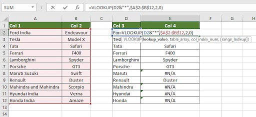{width=512 height=234}
*Using a wildcard in VLOOKUP to accommodate partial matches in column comparison.*
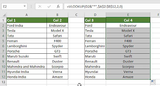{width=512 height=274}
*Results from VLOOKUP with a wildcard, showing matches based on partial text comparison.*4. IF Formula: Customizing Match/Mismatch Output
The IF formula provides a flexible way to compare two columns and display specific text or perform actions based on whether the values match or not.
Formula:
=IF(logical_test, value_if_true, value_if_false)
Comparing Columns with IF Formula:
To compare Column A and Column B and display “Same” if they match and “Different” if they don’t, use the formula: =IF(A2=B2, "Same", "Different").
{width=512 height=270}
*Applying the IF formula to compare columns and display custom "Same" or "Different" results.*This formula directly compares A2 and B2. If they are equal (TRUE), it returns “Same”; otherwise (FALSE), it returns “Different.” You can customize the “value_if_true” and “value_if_false” arguments to display any text or perform other calculations as needed.
5. EXACT Formula: Case-Sensitive Comparison
The EXACT formula is used for a case-sensitive comparison of two text strings. It returns TRUE if the strings are exactly the same (including case) and FALSE otherwise.
Formula:
=EXACT(text1, text2)
Case-Sensitive Column Comparison:
To compare Column A and Column B case-sensitively, use the formula: =EXACT(A2, B2).
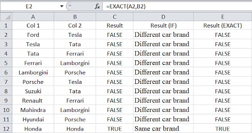{width=512 height=271}
*Using the EXACT formula to perform a case-sensitive comparison between two columns.*If the values in A2 and B2 are identical in both content and case, the formula will return TRUE. If there is any difference in case or content, it will return FALSE. Remember that “Apple” and “apple” will be considered different by the EXACT formula.
Choosing the Right Method for Your Scenario
The best method for comparing two columns in Excel depends on your specific needs and scenario. Here’s a guide to help you choose:
Scenario 1: Row-by-Row Comparison for Matches and Differences
For simple row-by-row comparisons to identify matches or differences, use:
-
Equals Operator (=): For basic TRUE/FALSE results.
=IF(A2 = B2, "Match", " ")=IF(A2<>B2, "No Match", " ")=IF(A2 = B2, "Match", "No Match")
-
EXACT Formula: For case-sensitive row-by-row comparisons.
=IF(EXACT(A2, B2), "Match", " ")=IF(EXACT(A2, B2), "Match", "No Match")
Scenario 2: Comparing Multiple Columns for Row Matches
To compare more than two columns and check for matches across rows, use:
-
AND with Equals: For checking if all specified columns in a row have identical values.
=IF(AND(A2=B2, A2=C2), "Complete Match", " ")
-
COUNTIF: To check if a specific number of columns in a row match a particular value (e.g., the value in the first column).
=IF(COUNTIF($A2:$E2, $A2)=4, "Complete Match", " ")(Here, 4 is the number of columns you are comparing, excluding the first column itself which is being counted).
Scenario 3: Finding Unique Values (Values in One Column Not in Another)
To identify values present in Column A but not in Column B, use:
-
COUNTIF: To count occurrences of values from Column A in Column B. If the count is 0, the value is unique to Column A.
=IF(COUNTIF($B:$B, $A2)=0, "Not in Column B", "")
-
MATCH with ISERROR: To check if a value from Column A can be found in Column B. ISERROR combined with MATCH indicates if a match was not found.
=IF(ISERROR(MATCH($A2, $B$2:$B$10, 0)), "Not in Column B", "")
-
Combined Match/Present Output: To show both matches and unique values in one formula.
=IF(COUNTIF($B:$B, $A2)=0, "Not in Column B", "Present in Column B")
Scenario 4: Comparing Two Lists and Extracting Matching Data
To compare two lists and retrieve matching data from the second list based on matches in the first, use:
-
VLOOKUP: To find and retrieve corresponding data from a second list based on values in the first list.
=VLOOKUP(D2, $A$2:$B$6, 2, FALSE)
-
INDEX MATCH: A more flexible alternative to VLOOKUP, especially when the lookup column is not the first column in the lookup range.
=INDEX($B$2:$B$6, MATCH($D2, $A$2:$A$6, 0))
-
XLOOKUP: A modern and more powerful lookup function, replacing both VLOOKUP and INDEX/MATCH in newer Excel versions.
=XLOOKUP(D2, $A$2:$A$6, $B$2:$B$6)
(Note: In these formulas, D2 represents the lookup value from your first list, and $A$2:$B$6 and $A$2:$A$6:$B$2:$B$6 represent the lookup range and return range from your second list.)
Scenario 5: Highlighting Row Matches and Differences Visually
To visually highlight entire rows that have matches or differences across columns, use Conditional Formatting with formulas:
- Select the Data Range: Select the range of data you want to compare.
- Conditional Formatting – New Rule: Go to “Home” > “Conditional Formatting” > “New Rule.”
- Use a Formula: Choose “Use a formula to determine which cells to format.”
- Enter Formula:
- Highlight Row Matches:
=AND($A2=$B2, $A2=$C2)(for highlighting rows where columns A, B, and C match). - Highlight Row Differences: Use “Go To Special” > “Row Differences” as described below.
- Highlight Row Matches:
- Format: Set the desired formatting (fill color, etc.).
- Apply: Click “OK.”
Using “Go To Special” for Row Differences:
This built-in Excel feature quickly highlights cells in each row that are different from a comparison cell within the same row.
-
Select Columns: Select the columns you want to compare.
-
Go To Special: Press
Ctrl + G(orF5) to open the “Go To” dialog, then click “Special.” -
Choose Row Differences: Select “Row differences” and click “OK.”
Excel will select cells that differ from the first cell in each row within your selection. You can then apply fill color or other formatting to highlight these differences.
Frequently Asked Questions (FAQs)
1. What is the easiest way to compare two columns in Excel?
The easiest method is often using Conditional Formatting to highlight duplicate or unique values visually. Alternatively, using the equals operator (=) in a new column provides a straightforward row-by-row comparison with TRUE/FALSE results.
2. Can I compare two columns in Excel using INDEX-MATCH?
Yes, INDEX-MATCH is a powerful method to compare columns, especially when you need to retrieve related data based on matches or when VLOOKUP’s limitations are a factor. It offers more flexibility than VLOOKUP.
3. How can I compare multiple columns in Excel at once?
For comparing multiple columns, you can use Conditional Formatting to highlight duplicates or uniques across the selected range. Formulas using AND, OR, or COUNTIF can also be adapted to compare multiple columns based on specific criteria.
4. How do I compare two lists in Excel for matches?
You can compare two lists using functions like VLOOKUP, INDEX-MATCH, or XLOOKUP to find matching values and potentially retrieve related data. Conditional formatting can also help visually identify matches or unique entries between two lists.
5. How do I compare two columns and highlight duplicates in Excel?
To highlight duplicates in two columns:
- Select the two columns.
- Go to “Home” > “Conditional Formatting” > “Highlight Cells Rules” > “Duplicate Values.”
- Ensure “Duplicate” is selected and choose your desired formatting.
- Click “OK.”
Excel will then highlight all values that appear in both selected columns.
Next Steps in Your Excel Journey
Mastering column comparison in Excel is a fundamental skill for data analysis and manipulation. To further enhance your Excel proficiency, explore related topics like:
- Pivot Tables and Charts: Learn to summarize and visualize data dynamically, creating interactive dashboards for deeper insights.
- Advanced Excel Formulas: Delve into more complex formulas and functions for data manipulation, analysis, and automation.
- Data Analysis Techniques in Excel: Expand your understanding of statistical and analytical methods you can implement within Excel.
By continuing to learn and practice, you can unlock the full potential of Excel for data analysis and become more efficient and effective in your data-driven tasks.