How to Compare Two Excel Sheets for Matches: A Step-by-Step Guide

Manually comparing data across two Excel sheets can quickly become a tedious and time-consuming task, especially when dealing with large datasets. However, accurately identifying matching data between spreadsheets is crucial for various tasks, from reconciling accounts to verifying data integrity. Fortunately, Excel provides powerful built-in features and formulas to streamline this process and significantly enhance your efficiency.

In this guide, we will explore effective methods to compare two Excel sheets for matching data within the same workbook. We will cover step-by-step instructions using Excel’s functionalities to help you quickly pinpoint identical entries and manage your data more effectively.

We will delve into the following methods:

Leveraging the MATCH Function to identify matches.
Utilizing Conditional Formatting to highlight matched data visually.

Let’s dive in and discover how to make comparing Excel sheets for matches a breeze!

Compare Two Sheets for Matching Data within the Same Excel Workbook: Detailed Methods

Method 1: Using the MATCH Function to Find Matches

The MATCH function in Excel is a robust tool that searches for a specified item in a range of cells and returns the relative position of that item in the range. We can harness this function to determine if values from one sheet exist in another. Here’s how:

Prepare Your Worksheets: Ensure both Excel sheets you intend to compare are open within the same workbook. This allows for easy referencing between sheets.
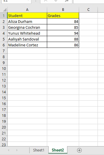
Insert a Helper Column: In the sheet where you want to display the comparison results (let’s say Sheet2), insert a new column next to the data you want to compare. This column will act as a “helper” column to show whether each item has a match in Sheet1.
Enter the MATCH Formula: In the first cell of your helper column (e.g., cell C2 in Sheet2), enter the following MATCH formula:
```
=MATCH(B2,Sheet1!B:B,0)
```
Let’s break down this formula:
- =MATCH(...): This initiates the MATCH function.
- B2: This is the lookup value – the value from cell B2 in Sheet2 that you are searching for in Sheet1. Adjust this to match the first cell containing data in the column you want to compare in Sheet2.
- Sheet1!B:B: This is the lookup array – it specifies the range to search within. Sheet1! refers to the worksheet named “Sheet1”, and B:B indicates that we are searching the entire column B of Sheet1. You can adjust the column letter if your data is in a different column in Sheet1.
- 0: This is the match type. 0 specifies an exact match – MATCH will only find values that are exactly the same as the lookup value.
Apply the Formula to the Entire Column: Press Enter. The cell will display either a number or #N/A.
- A Number: Indicates a match is found! The number represents the row number in Sheet1 where the matching value is located.
- #N/A: Means no match was found for the value from Sheet2 in Sheet1’s column B.
Use the fill handle (the small square at the bottom-right corner of the selected cell) to drag the formula down to apply it to all the rows in your data column in Sheet2. This will perform the comparison for each value in Sheet2 against Sheet1.

Now you have a clear indication in your helper column of which values from Sheet2 are present in Sheet1. You can filter or sort this helper column to isolate the matched or unmatched entries for further analysis.

Method 2: Highlighting Matched Data Using Conditional Formatting and MATCH

For a visual approach, you can use Conditional Formatting in combination with the MATCH function to directly highlight the matching data within your sheets. This method is excellent for quickly spotting matches.

Select Your Data Range: In Sheet2, select the range of cells containing the data you want to compare against Sheet1. For example, select cells B2 to B6 if those are the cells containing your data.
Enter the Conditional Formatting Formula: Go to the Home tab on the Excel ribbon, then click on Conditional Formatting > New Rule.

In the “New Formatting Rule” dialog box, select “Use a formula to determine which cells to format”. In the “Format values where this formula is true” box, enter the following formula:
```
=ISNUMBER(MATCH(B2,Sheet1!$B$2:$B$6,0))
```
Let’s break down this formula and how it works with conditional formatting:
- =ISNUMBER(...): The ISNUMBER function checks if a value is a number. It returns TRUE if the value is a number and FALSE otherwise.
- MATCH(B2, Sheet1!$B$2:$B$6, 0): This is the same MATCH function we used earlier. It attempts to find the value of cell B2 (in Sheet2) within the range $B$2:$B$6 of Sheet1.
- Sheet1!$B$2:$B$6: This is the specific range in Sheet1 (Column B, rows 2 through 6) to search for matches. Important: Note the absolute references $B$2:$B$6. The dollar signs ($) ensure that this range remains fixed when the conditional formatting rule is applied to other cells. Adjust this range to accurately reflect the data range in Sheet1 you are comparing against.
- 0: Specifies an exact match.
The entire formula =ISNUMBER(MATCH(B2,Sheet1!$B$2:$B$6,0)) will return TRUE if MATCH finds a match (and thus returns a number – the row position), and FALSE if MATCH returns #N/A (no match). Conditional Formatting will then apply formatting only to cells where this formula evaluates to TRUE.
Set the Formatting: Click the Format button in the “New Formatting Rule” dialog box. Choose the formatting style you want to apply to the matched cells (e.g., fill color, font style). Click OK to set the format and then OK again to close the “New Formatting Rule” dialog box.
Apply Conditional Formatting: Excel will automatically apply the conditional formatting to your selected range. You should now see the cells in Sheet2 that have matching values in Sheet1 highlighted according to the format you selected.
Refine and Customize: You can adjust the conditional formatting rules at any time by going to Home > Conditional Formatting > Manage Rules. Here you can edit the formula, change the formatting, or adjust the range to which the rule applies.
View Highlighted Matches: After applying conditional formatting, visually scan your Sheet2. The highlighted cells are those containing data that matches entries in Sheet1 within the specified columns.

By using Conditional Formatting with the MATCH function, you can instantly visualize matching data points across your Excel sheets, making data comparison and analysis much more intuitive and efficient.

Final Thoughts on Comparing Two Excel Sheets for Matches

These methods, utilizing the MATCH function and Conditional Formatting, offer efficient ways to compare data for matches between two Excel sheets within the same workbook. Whether you prefer to see the row position of matches or visually highlight them, Excel provides the tools to simplify your data comparison tasks.

Explore more step-by-step Excel tutorials and tips by visiting Simple Sheets! Check out related articles below and our Facebook Page for Excel and Google Sheets templates to further enhance your spreadsheet skills!

Frequently Asked Questions about Comparing Two Excel Sheets for Matches

Can I use INDEX MATCH across different sheets?

Yes! The INDEX MATCH combination is incredibly versatile and works seamlessly across different sheets within the same Excel workbook, or even across different workbooks if they are open. This makes it highly useful for consolidating and comparing data from various sources within Excel. The MATCH function part of INDEX MATCH (as we used standalone above) is specifically designed to find matches across sheets.

Is VLOOKUP suitable for comparing two sheets?

While VLOOKUP can retrieve data from another sheet based on a lookup value, it’s not directly used for comparing two sheets for matches in the same way as MATCH or Conditional Formatting. VLOOKUP is more about pulling related information from one sheet to another. However, you could indirectly use VLOOKUP to achieve a comparison by using it to check if values from one sheet exist in another, similar to how we used MATCH, but MATCH is generally more efficient and flexible for direct comparison tasks.

What is the best formula for matching values in Excel?

The MATCH function is often considered the best formula specifically for finding matching values in Excel when you need to know where a value is located within a range (its relative position). For simply determining if a value exists in another range, combining MATCH with ISNUMBER (as shown in Conditional Formatting) is highly effective. For more complex lookups and retrieving associated data, INDEX MATCH (which includes MATCH) is a superior and more flexible alternative to VLOOKUP, especially for larger datasets or when dealing with columns that might be reordered.

How to Compare Two Excel Sheets

SUM Index-Match: What is it, and How do I use it?

The Top 5 Google Sheets Formulas You Need to Know