How to Compare Two Columns in Excel for Matches and Highlight: Your Comprehensive Guide

Excel is a powerhouse for data management, and one common task is comparing two columns to identify matching entries and highlight them for better data analysis. Whether you’re reconciling lists, checking for duplicates, or simply need to see common items at a glance, Excel offers several efficient methods. This guide will walk you through various techniques to compare two columns in Excel for matches and highlight, ensuring you can choose the best approach for your specific needs.

We’ll cover everything from simple formulas for basic comparisons to more advanced conditional formatting techniques that visually emphasize matches. By the end of this tutorial, you’ll be proficient in comparing columns and highlighting matches in Excel, boosting your data analysis efficiency.

Understanding Different Comparison Scenarios

Before diving into the methods, it’s important to understand the different scenarios you might encounter when you compare two columns in Excel for matches and highlight:

• Exact Row Match: You need to compare cells in the same row across two columns and determine if they are identical.
• Matching Data Points (Any Row): You want to find and highlight data points that appear in both columns, regardless of their row position.
• Mismatched Data Points: You need to identify and highlight data points that are unique to each column, indicating differences between the lists.
• Finding Missing Data: You want to check if values from one column exist in another and identify the missing values.
• Pulling Matching Data: You need to retrieve corresponding data from another column based on matches found in the comparison.

Let’s explore the methods for each of these scenarios.

1. Comparing Two Columns for Exact Row Matches

This is the simplest form of comparison where you check if the data in the same row of two columns matches.

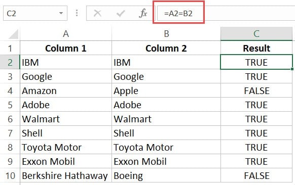
1.1. Using a Simple Formula to Check for Matches

You can use a basic formula to return TRUE if the cells in the same row of two columns are identical, and FALSE otherwise.

Example: Suppose you have company names in Column A and Column B, and you want to check for matches row by row.

1. In cell C2 (or any empty column in the same row), enter the formula: =A2=B2

2. Drag the fill handle (the small square at the bottom-right of the cell) down to apply the formula to the rest of the rows.

This formula directly compares the content of cell A2 with cell B2. If they are the same, it returns TRUE; otherwise, it returns FALSE.

1.2. Using the IF Formula for Descriptive Results

For more descriptive results like “Match” or “Mismatch,” you can use the IF formula.

Example: Using the same company name list, let’s get “Match” or “Mismatch” as results.

1. In cell C2, enter the formula: =IF(A2=B2,"Match","Mismatch")
2. Drag the fill handle down to apply the formula to all rows.

This formula checks if A2 equals B2. If TRUE, it returns “Match”; if FALSE, it returns “Mismatch.”

Case-Sensitive Comparison: If you need a case-sensitive comparison (e.g., “Apple” and “apple” should be considered different), use the EXACT function within the IF formula:

=IF(EXACT(A2,B2),"Match","Mismatch")

1.3. Highlighting Rows with Matching Data Using Conditional Formatting

To visually highlight entire rows where the data in two columns match, use Conditional Formatting.

Steps:

1. Select your entire dataset (including headers if applicable).

2. Go to Home tab > Conditional Formatting > New Rule.

3. In the “New Formatting Rule” dialog box, select “Use a formula to determine which cells to format.”

4. Enter the formula: =$A1=$B1 (adjust the row number if your data starts from a different row). Important: Ensure you select the first row of your data range before setting up conditional formatting.

5. Click the Format button, choose your desired formatting (e.g., fill color), and click OK twice.

This will highlight all rows where the values in column A and column B of the same row are identical.

2. Comparing Two Columns and Highlighting Matches Across Columns

If you need to find matches that appear in both columns, regardless of their row position, you can use the “Duplicate Values” feature in Conditional Formatting.

2.1. Highlighting Matching Data Points in Two Columns

This method is useful when you have two lists and want to highlight the items that are present in both.

Steps:

1. Select both columns of data you want to compare.

2. Go to Home tab > Conditional Formatting > Highlight Cells Rules > Duplicate Values.

3. In the “Duplicate Values” dialog box, ensure “Duplicate” is selected in the dropdown. Choose your desired formatting and click OK.

This will highlight all values that appear in both Column A and Column B. Note that the “Duplicate Values” rule is not case-sensitive.

2.2. Highlighting Mismatched Data Points (Unique Values)

Conversely, you can highlight data points that are unique to each column, effectively showing the differences between the two lists.

Steps:

1. Select both columns of data.

2. Go to Home tab > Conditional Formatting > Highlight Cells Rules > Duplicate Values.

3. In the “Duplicate Values” dialog box, change the dropdown from “Duplicate” to “Unique”. Choose your formatting and click OK.

This will highlight values that are present in one column but not the other, showcasing the unique entries in each list.

3. Comparing Two Columns to Find Missing Data Points

To determine if data points from one column are present in another and identify the missing ones, you can use lookup formulas like VLOOKUP or MATCH.

3.1. Using VLOOKUP to Find Missing Values

VLOOKUP can check if a value from one column exists in another. Combined with ISERROR, it can effectively identify missing data.

Example: Suppose you want to find companies in Column A that are NOT present in Column B.

1. In cell C2, enter the formula: =ISERROR(VLOOKUP(A2,$B$2:$B$10,1,FALSE)) (adjust the range $B$2:$B$10 to cover all of Column B).

2. Drag the fill handle down. TRUE indicates the company in Column A is NOT found in Column B (missing).

VLOOKUP(A2,$B$2:$B$10,1,FALSE) attempts to find the value of A2 in the range B2:B10. If not found, it returns an error #N/A. ISERROR then checks for this error. If there is an error (TRUE), it means the value is missing from Column B.

3.2. Using MATCH to Find Missing Values

The MATCH function is another powerful tool for this purpose, often considered more flexible than VLOOKUP.

Example: Using the same scenario, find companies in Column A missing from Column B.

1. In cell C2, enter the formula: =ISNA(MATCH(A2,$B$2:$B$10,0))
2. Drag the fill handle down. TRUE indicates the company is missing.

Alternatively, to get TRUE for values that ARE present (and FALSE for missing), you can use:

=ISNUMBER(MATCH(A2,$B$2:$B$10,0))

or

=NOT(ISNA(MATCH(A2,$B$2:$B$10,0)))

MATCH(A2,$B$2:$B$10,0) tries to find the position of A2 in B2:B10. If found, it returns the position (a number); if not, it returns #N/A. ISNA checks for the #N/A error.

4. Comparing Two Columns and Pulling Matching Data

In situations where you have related data in columns and want to retrieve information based on matches, lookup formulas are essential.

4.1. Pulling Exact Matching Data

If you have a lookup column and a value column, and you want to fetch the value corresponding to a match in another column, VLOOKUP or INDEX/MATCH are ideal.

Example: Column A has company names, Column B has Market Valuation. You have a list of companies in Column D, and you want to pull their Market Valuation from Columns A and B.

1. In cell E2, enter the formula: =VLOOKUP(D2,$A$2:$B$14,2,FALSE) (or =INDEX($B$2:$B$14,MATCH(D2,$A$2:$A$14,0))). Adjust ranges as needed.

2. Drag the fill handle down.

VLOOKUP(D2,$A$2:$B$14,2,FALSE) searches for D2 in the first column of the range A2:B14 and returns the value from the 2nd column (Valuation) in the same row. INDEX/MATCH provides the same result, with MATCH finding the row number and INDEX fetching the value from that row in the Valuation column.

4.2. Pulling Partial Matching Data

When dealing with lists where names might not be exactly identical (e.g., “JPMorgan” vs. “JPMorgan Chase”), you can use wildcard characters with VLOOKUP or INDEX/MATCH for partial matches.

Example: Column A and B are the same as above, but Column D has abbreviated company names.

1. In cell E2, enter: =VLOOKUP("*"&D2&"*",$A$2:$B$14,2,FALSE) (or =INDEX($B$2:$B$14,MATCH("*"&D2&"*",$A$2:$A$14,0))).

2. Drag down.

The asterisks "*" are wildcard characters that match any sequence of characters. "*"&D2&"*" means “find any value in Column A that contains the text in D2.”

Conclusion

Comparing two columns in Excel for matches and highlighting is a fundamental skill for data analysis. This guide has provided you with a range of methods, from simple formulas to conditional formatting and powerful lookup functions. Choose the technique that best suits your specific comparison needs and data structure. By mastering these methods, you’ll significantly enhance your ability to analyze and manage data effectively in Excel. Whether you need to highlight exact matches, find differences, or pull related data, Excel offers the tools to streamline your workflow and gain valuable insights from your spreadsheets.