Excel Compare Columns for Differences: Your Comprehensive Guide

Comparing columns in Excel to identify differences is a frequent task for data analysis, list management, and ensuring data integrity. While Excel offers several built-in features, knowing the right techniques can significantly streamline your workflow. This guide explores various methods to Excel Compare Columns For Differences, ranging from simple formulas to advanced features, ensuring you can pinpoint discrepancies effectively.

How to Compare Two Columns in Excel for Differences Row-by-Row

When you need to scrutinize data on a row-by-row basis, Excel provides straightforward methods to highlight differences. The IF function is a powerful tool for this, allowing you to compare corresponding cells in two columns and flag any discrepancies.

Example 1: Identifying Differences in Two Columns within the Same Row

To begin, let’s use the IF function to compare two columns and highlight where values differ in each row. This is useful for ensuring data consistency across columns for related entries.

Formula for Differences:

To find cells within the same row that contain different values, use the following IF formula. Enter this formula in a spare column in the same row as your data, and then drag the fill handle (the small square at the bottom-right of the cell) down to apply it to all rows.

=IF(A2<>B2,"Difference","")

In this formula:

• A2<>B2 checks if the value in cell A2 is not equal to the value in cell B2.
• "Difference" is the text that will be displayed if the condition is true (i.e., the values are different).
• "" (empty string) is displayed if the values are the same.

Example with Matches and Differences:

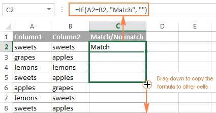
You can easily modify the formula to identify both matches and differences simultaneously:

=IF(A2<>B2,"Difference","Match")

Or, to reverse the output:

=IF(A2=B2,"Match","Difference")

The results clearly show “Difference” where discrepancies exist and “Match” where the values are identical, accommodating numbers, dates, times, and text strings effectively.

Tip: For large datasets, consider using Excel’s Advanced Filter to quickly filter rows where differences occur between two columns. This can help you focus only on the rows that require attention.

Example 2: Case-Sensitive Difference Detection

Standard Excel comparisons are case-insensitive. If you need to differentiate between text based on case, the EXACT function is essential.

Formula for Case-Sensitive Differences:

To find differences that are case-sensitive, combine the EXACT function with the IF function:

=IF(EXACT(A2, B2), "", "Case Difference")

In this case:

• EXACT(A2, B2) returns TRUE if A2 and B2 are exactly the same, including case, and FALSE otherwise.
• "" (empty string) is displayed if the values are exactly the same (case-sensitive match).
• "Case Difference" is displayed if the values are different, or different only in case.

By using the EXACT function, you can ensure that your comparison is precise, especially when case sensitivity is critical to your data analysis.

Comparing Multiple Columns for Differences in the Same Row

Excel also allows you to compare multiple columns within the same row to find differences. This is useful when you have datasets with several attributes for each entry and need to ensure consistency across these attributes.

Example 1: Identifying Rows with Any Differences Across Multiple Columns

If you want to find rows where at least one column differs from the others in the same row, you can use a combination of IF and OR functions.

Formula for Any Difference in Multiple Columns:

For comparing columns A, B, and C in the same row, the formula is:

=IF(OR(A2<>B2, B2<>C2, A2<>C2), "Difference", "")

This formula checks if any of the pairwise comparisons (A2 vs B2, B2 vs C2, A2 vs C2) results in a difference. If any difference is found, it flags “Difference”.

For a larger number of columns, constructing a long OR statement can become cumbersome. A more scalable approach involves using COUNTIF in conjunction with IF.

Alternative Formula using COUNTIF for Multiple Columns:

=IF(COUNTIF($A2:$E2, $A2)=5, "", "Difference")

Here, we assume you are comparing 5 columns (A to E).

• COUNTIF($A2:$E2, $A2) counts how many times the value in A2 appears within the range A2:E2.
• If the count is 5, it means all cells in the range A2:E2 are the same as A2 (no difference).
• If the count is not 5, it indicates at least one cell is different, and “Difference” is displayed.

This COUNTIF method is more efficient for comparing a larger number of columns as it avoids lengthy nested OR conditions.

Example 2: Finding Rows with Differences Across All Columns

Conversely, you might need to identify rows where all columns have different values from each other. This is less common but can be important in specific data analysis scenarios.

While a direct formula to check “all different” can be complex, you can adapt the COUNTIF approach to identify rows where values are not consistently the same across all columns, which indirectly highlights rows with differences.

How to Compare Two Columns for Differences Between Lists

Often, you’ll have two separate lists in different columns and need to find values that are present in one list but not in the other. This is crucial for tasks like identifying missing items, unique entries, or discrepancies between datasets.

Formula using COUNTIF to Find Differences Between Two Lists:

Suppose you have List 1 in column A and List 2 in column B. To find values in List 1 that are not present in List 2, use the following formula in a column next to List 1:

=IF(COUNTIF($B:$B, $A2)=0, "Unique to List 1", "")

In this formula:

• COUNTIF($B:$B, $A2) counts how many times the value in cell A2 appears in the entire column B (List 2).
• If the count is 0, it means the value from A2 is not found in List 2, indicating it’s unique to List 1.
• "Unique to List 1" is displayed if the value is not found in List 2.
• "" (empty string) is displayed if the value is found in List 2 (i.e., it’s not unique to List 1).

Tip: For performance optimization in large datasets, instead of referencing entire columns ($B:$B), specify a definite range (e.g., $B$2:$B$1000) to limit the scope of the COUNTIF function.

Alternative Formulas using MATCH and ISERROR:

You can achieve the same result using a combination of MATCH and ISERROR functions:

=IF(ISERROR(MATCH($A2,$B$2:$B$10,0)),"Unique to List 1","")

Or using an array formula with SUM (remember to press Ctrl + Shift + Enter):

=IF(SUM(--($B$2:$B$10=$A2))=0, "Unique to List 1", "")

These formulas check if a value from List 1 can be found in List 2. If MATCH results in an error (ISERROR is TRUE), it means the value is not found, and it’s unique to List 1.

To identify values unique to List 2 (present in List 2 but not in List 1), simply reverse the columns in the formulas:

=IF(COUNTIF($A:$A, $B2)=0, "Unique to List 2", "")

Highlighting Differences in Excel Columns Visually

While formulas help identify differences textually, conditional formatting allows you to visually highlight these discrepancies directly in your worksheet, making it easier to spot patterns and anomalies.

Example 1: Highlighting Row Differences

To visually emphasize differences between two columns on a row-by-row basis, conditional formatting is ideal.

Steps to Highlight Differences in Each Row:

1. Select the range of cells you want to compare (e.g., column A and B data rows).
2. Go to Home tab > Conditional Formatting > New Rule.
3. Choose “Use a formula to determine which cells to format”.
4. Enter the formula to find differences: =$A2<>$B2 (assuming row 2 is your first data row). Ensure you use a relative row reference (no $ before the row number).
5. Click Format to choose a highlighting style (e.g., fill color) and click OK twice.

Excel will now highlight cells in column A where the value differs from the corresponding cell in column B in the same row, providing a clear visual representation of the differences.

Example 2: Highlighting Unique Entries Between Two Lists

Conditional formatting can also be used to highlight entries that are unique to each list when comparing two columns as lists.

Highlighting Unique Values in List 1 (Column A):

1. Select List 1 (e.g., cells A2:A6).
2. Go to Conditional Formatting > New Rule > “Use a formula…”.
3. Enter the formula: =COUNTIF($C$2:$C$5, $A2)=0 (assuming List 2 is in C2:C5).
4. Set your desired formatting and click OK.

Highlighting Unique Values in List 2 (Column C):

1. Select List 2 (e.g., cells C2:C5).
2. Create a new conditional formatting rule with the formula: =COUNTIF($A$2:$A$6, $C2)=0 (referencing List 1 range A2:A6).
3. Choose formatting and apply.

This setup visually distinguishes items that are exclusive to each list, making it easy to identify unique entries and differences between your datasets.

Example 3: Highlighting Differences in Multiple Columns Row-wise using “Go To Special”

For a quick, formula-free method to highlight differences across multiple columns in each row, Excel’s “Go To Special” feature is invaluable.

Steps to Highlight Row Differences with “Go To Special”:

1. Select the range of cells across the columns you want to compare (e.g., A2:C8). The top-left cell will be the “comparison cell.”
2. Navigate to Home tab > Editing group > Find & Select > Go To Special….
3. In the “Go To Special” dialog, select “Row differences” and click OK.

Excel will select all cells in each row that are different from the value in the comparison cell (the first cell in the selected range of each row). You can then apply a fill color to these selected cells to highlight the differences.

This method is exceptionally fast for visually spotting differences in rows without needing to set up formulas.

Formula-Free Column Comparison Using Ablebits Compare Tables Add-in

For users seeking a more streamlined, formula-free approach to compare columns for differences, the Compare Two Tables add-in from Ablebits offers a powerful solution. This tool simplifies the process of identifying both matches and differences between two lists or tables.

Using Compare Tables Add-in to Find Differences:

1. Install and open the Ablebits Ultimate Suite add-in in Excel.
2. Click the Compare Tables button on the Ablebits Data tab.
3. Select your first list or column (Table 1) and click Next.

4. Select your second list or column (Table 2) and click Next.

5. Choose the type of data to find. To find differences (unique values), select Unique values. You can choose to find values unique to Table 1, Table 2, or both. Click Next.

6. Specify the columns you want to compare. For simple column comparison, select the respective columns from Table 1 and Table 2. Click Next.

7. Choose how you want to handle the found differences. Options include highlighting with color or adding a “Status” column to label differences. For highlighting, select Highlight with color and choose a color. Click Finish.

The add-in will then process your lists and visually highlight or label the differences based on your chosen settings, providing a quick and efficient way to compare columns without manual formula setup.

Conclusion

Comparing columns in Excel to find differences is a fundamental skill for data analysis and management. Whether you prefer using Excel’s built-in formulas like IF, COUNTIF, and EXACT, leveraging conditional formatting for visual cues, or opting for efficient add-ins like Ablebits Compare Tables, Excel offers a range of tools to suit your needs. By understanding these methods, you can effectively identify discrepancies, ensure data accuracy, and streamline your Excel workflows. Explore these techniques to enhance your data comparison capabilities and achieve greater insights from your spreadsheets.

Downloadable Resources:

Excel Column Comparison Examples (.xlsx file)
Ablebits Ultimate Suite – Trial Version (.exe file)

Further Reading:

How to Compare Two Columns Using VLOOKUP in Excel
Excel Conditional Formatting Formulas: A Step-by-Step Guide
Using Excel Advanced Filter to Compare Columns