Excel Compare 2 Sheets: Unveiling Differences and Boosting Efficiency

In today’s data-driven world, Microsoft Excel remains an indispensable tool for managing and analyzing information. Whether you’re tracking sales figures, managing project data, or organizing research, you often find yourself working with multiple spreadsheets. A common challenge arises when you need to compare two Excel sheets to identify changes, discrepancies, or simply understand how data has evolved. This comprehensive guide will explore various methods to effectively “Excel Compare 2 Sheets”, empowering you to pinpoint differences, streamline your workflow, and ensure data accuracy.

Comparing two Excel sheets isn’t just about finding errors; it’s a powerful technique for:

Version Control: Quickly see what’s changed between different versions of a report or dataset.
Data Auditing: Verify data integrity by comparing source and destination sheets after data migration or manipulation.
Collaboration: Understand contributions from multiple team members working on the same spreadsheet.
Troubleshooting: Identify inconsistencies in formulas, data entry errors, or formatting discrepancies.
Merging Data: Prepare for data consolidation by understanding the variations between sheets.

From simple visual checks to advanced third-party tools, this article will equip you with the knowledge and techniques to master the art of “excel compare 2 sheets” and elevate your Excel proficiency. Let’s delve into the methods that can transform how you analyze and manage your spreadsheet data.

Side-by-Side Viewing: A Visual Approach to Excel Sheet Comparison

For a quick, initial comparison, especially with smaller datasets, leveraging Excel’s built-in “View Side by Side” feature offers a straightforward visual method to “excel compare 2 sheets”. This technique allows you to arrange two Excel windows adjacent to each other, facilitating a direct visual scan for differences.

Comparing Two Excel Workbooks Side by Side

Imagine you have monthly sales reports in two separate Excel files and need to quickly grasp product performance changes. The “View Side by Side” mode is your efficient solution.

Open Your Workbooks: Begin by opening both Excel files you intend to compare.
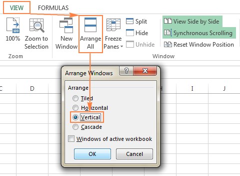
Activate “View Side by Side”: Navigate to the “View” tab on the Excel ribbon. In the “Window” group, locate and click the “View Side by Side” button.

By default, Excel will display the two workbooks horizontally, one above the other.

To arrange them vertically, positioned next to each other, click the “Arrange All” button within the “Window” group on the “View” tab and select “Vertical”.

This vertical arrangement provides an optimal layout for comparing data columns across the two sheets.

To enhance the comparison process, ensure “Synchronous Scrolling” is enabled. This feature, located directly beneath the “View Side by Side” button in the “Window” group of the “View” tab, typically activates automatically with “View Side by Side”. With synchronous scrolling, scrolling in one window will simultaneously scroll the other, ensuring you are always viewing corresponding rows.

For a more detailed guide on this feature, refer to “View Excel workbooks side by side.”

Viewing Multiple Excel Windows Simultaneously

If you need to compare more than two Excel files, Excel allows you to arrange multiple windows side by side. After opening all the relevant workbooks, clicking “View Side by Side” will open the “Compare Side by Side” dialog box. Here, you can select which files to display alongside the currently active workbook.

Alternatively, to view all open Excel files at once, utilize the “Arrange All” button in the “Window” group of the “View” tab. Choose from arrangements like “Tiled,” “Horizontal,” “Vertical,” or “Cascade” to best suit your viewing needs.

Comparing Two Sheets Within the Same Workbook

Often, the two sheets you wish to compare reside within the same Excel workbook. To view these sheets side by side, follow these steps:

Open a New Window: Open your Excel file, then go to the “View” tab and, in the “Window” group, click “New Window”. This action opens a second window displaying the same workbook.
Enable Side by Side View: Click the “View Side by Side” button on the ribbon. Excel will now arrange the two windows of the same workbook side by side.
Select Sheets: In each window, navigate to and select the specific sheet you want to compare. One window will display Sheet 1, and the other will display Sheet 2, allowing for direct comparison.

This “View Side by Side” method is ideal for quick visual inspections but may become cumbersome for large datasets or when seeking precise difference identification. For more detailed and automated comparisons, explore the following methods.

Formula-Based Difference Reports: Identifying Value Discrepancies in Excel Sheets

For a more analytical approach to “excel compare 2 sheets”, using Excel formulas to generate a difference report provides a structured way to identify cells with differing values. This method outputs a new worksheet that highlights the specific discrepancies.

To create a difference report using formulas, follow these steps:

Open a New Sheet: In your Excel workbook, insert a new, blank worksheet. This sheet will serve as your difference report.
Enter the Comparison Formula: In cell A1 of the new sheet, enter the following formula:

=IF(Sheet1!A1 <> Sheet2!A1, "Sheet1:"&Sheet1!A1&" vs Sheet2:"&Sheet2!A1, "")

This formula checks if the value in cell A1 of “Sheet1” is different from the value in cell A1 of “Sheet2”. If they differ, it displays a text string indicating the values from both sheets. If they are the same, it leaves the cell blank.
Apply the Formula to the Entire Range: Drag the fill handle (the small square at the bottom-right corner of the selected cell) down and to the right to copy the formula across the range of cells you need to compare. This automatically adjusts the cell references (A1, B1, C1, A2, etc.) to compare corresponding cells in “Sheet1” and “Sheet2”.

The resulting difference report sheet will look similar to this:

As shown, the difference report clearly outlines cells where values diverge, displaying the values from both sheets for easy comparison. Note that dates, as seen in cell C4 of the example, might be represented by their serial numbers in the difference report due to Excel’s internal date storage. While functional, this format may not be ideal for intuitively analyzing date differences.

This formula method is effective for value comparison but has limitations. It does not account for differences in formulas, cell formatting, or structural changes like added or deleted rows and columns. For more comprehensive comparisons, consider conditional formatting or dedicated comparison tools.

Conditional Formatting: Visually Highlighting Differences Between Excel Sheets

To enhance visual difference detection when you “excel compare 2 sheets”, Excel’s conditional formatting feature offers a powerful way to automatically highlight cells with differing values. This method color-codes the discrepancies directly within one of your worksheets, making them immediately apparent.

Here’s how to highlight differences using conditional formatting:

Select the Data Range: In the worksheet where you want to visually highlight the differences, select the entire range of cells you wish to compare. Start by clicking the top-left cell of your data range (usually A1) and press Ctrl + Shift + End to extend the selection to the last used cell in your sheet.
Create a New Conditional Formatting Rule: Navigate to the “Home” tab on the Excel ribbon. In the “Styles” group, click “Conditional Formatting”, then select “New Rule”.
Use a Formula to Determine Formatting: In the “New Formatting Rule” dialog box, choose “Use a formula to determine which cells to format”.
Enter the Formula: In the “Format values where this formula is true” box, enter the following formula:

=A1<>Sheet2!A1

Ensure you replace “Sheet2” with the actual name of the sheet you are comparing against. This formula will evaluate to TRUE for any cell in your selected range where the value is not equal to the corresponding cell in “Sheet2”.
Set the Formatting: Click the “Format…” button to choose how you want the different cells to be highlighted. You can change the fill color, font style, border, and more. Select your desired formatting and click “OK” in both the “Format Cells” and “New Formatting Rule” dialog boxes.

Excel will now apply the conditional formatting rule to your selected range, instantly highlighting all cells that contain values different from their corresponding cells in “Sheet2”.

For a more in-depth guide on conditional formatting, see “Excel conditional formatting based on another cell value.”

While conditional formatting provides a visually effective way to highlight value differences, it shares similar limitations with the formula method. It primarily focuses on value discrepancies and does not detect differences in formulas, formatting, or structural changes. Furthermore, adding or deleting rows or columns in one sheet can misalign the comparison, marking subsequent rows/columns incorrectly. For a comprehensive comparison that addresses these limitations, consider the “Compare and Merge Shared Workbook” feature or explore specialized third-party tools.

Compare and Merge Shared Workbook: Tracking Changes in Collaborative Excel Files

When collaboration is key and multiple users are working on different copies of the same Excel workbook, the “Compare and Merge Workbooks” feature becomes invaluable for managing and consolidating changes. This feature is specifically designed for merging versions of a shared workbook, allowing you to review and incorporate edits from various users into a single master file.

Before utilizing “Compare and Merge Workbooks”, ensure these preparatory steps are taken:

Share the Workbook: The original workbook must be shared before copies are distributed for editing. To share, click the “Share Workbook” button on the “Review” tab, within the “Changes” group. Check the box labeled “Allow changes by more than one user at the same time…” and click “OK”. Excel may prompt you to save the workbook in a shared location. Enabling “Track Changes” automatically shares the workbook as well.
Save Copies with Unique Names: Each user editing the shared workbook must save their copy with a distinct filename (.xls or .xlsx format). This ensures that each set of changes can be identified and merged correctly.

With these preparations complete, you are ready to merge the copies back into the primary shared workbook.

1. Enabling the “Compare and Merge Workbooks” Command

Although the “Compare and Merge Workbooks” functionality is available in Excel versions from 2010 through Microsoft 365, it is not readily accessible in the default Excel ribbon or Quick Access Toolbar. To add it to your Quick Access Toolbar for easy access:

Access Excel Options: Click the dropdown arrow at the end of the Quick Access Toolbar and select “More Commands…”.
Choose Commands From “All Commands”: In the “Excel Options” dialog box, under “Choose commands from:”, select “All Commands”.
Add “Compare and Merge Workbooks”: Scroll down the list of commands to find “Compare and Merge Workbooks”. Select it and click the “Add >>” button to move it to the right-hand section, which lists commands in your Quick Access Toolbar.
Confirm Changes: Click “OK” to close the “Excel Options” dialog box. The “Compare and Merge Workbooks” command icon will now be visible in your Quick Access Toolbar.

2. Performing the Workbook Comparison and Merge

Once the command is added and all users have saved their copies of the shared workbook, you can proceed with merging these copies:

Open the Primary Workbook: Open the original, shared version of the Excel workbook.
Initiate Merge: Click the “Compare and Merge Workbooks” command icon in your Quick Access Toolbar.
Select Copies to Merge: In the dialog box that appears, select the copies of the shared workbook you wish to merge. To select multiple copies, hold down the Shift key while clicking on the filenames. Click “OK” to begin the merge process.

Excel will then merge the changes from each selected copy into the primary workbook.

3. Reviewing Merged Changes

To effectively review all the edits made by different users, utilize Excel’s “Track Changes” feature:

Highlight Changes: Go to the “Review” tab, “Changes” group, and click “Track Changes” > “Highlight Changes…”.
Configure Highlight Settings: In the “Highlight Changes” dialog box, set the following:
- When: Select “All” to review all changes made.
- Who: Select “Everyone” to see changes from all users.
- Where: Clear the “Where” box to review changes across the entire workbook.
- Highlight changes on screen: Ensure this box is checked to visually highlight the changes.
- Click “OK”.

Excel will highlight column letters and row numbers in dark red to indicate rows and columns with changes. At the cell level, edits from different users are marked with different colors. Hovering over a highlighted cell will display information about who made the change and when.

Important Note: The “Compare and Merge Workbooks” feature is specifically designed for merging copies of a shared workbook. It will not work for comparing and merging unrelated Excel files. If the command is greyed out, ensure you are working with the original shared workbook and attempting to merge copies of it.

While “Compare and Merge Workbooks” is excellent for collaborative scenarios, it is limited to tracking changes within a shared workbook framework and may not provide the detailed comparison and merging capabilities needed for general “excel compare 2 sheets” tasks. For advanced comparison needs, third-party tools offer more comprehensive solutions.

Third-Party Tools for Advanced Excel File Comparison

While Excel’s built-in features offer basic to intermediate capabilities to “excel compare 2 sheets”, they often fall short when it comes to comprehensive comparisons, particularly when dealing with complex workbooks or needing to identify all types of differences – values, formulas, formatting, and structural changes. Third-party tools are designed to bridge this gap, offering advanced functionalities for in-depth Excel file comparison and merging.

These specialized tools often provide:

Comprehensive Difference Detection: Identify discrepancies in values, formulas, cell formatting, sheet structure (added/deleted rows/columns), and even VBA code.
Detailed Reporting: Generate in-depth reports highlighting all types of differences found, often with visual aids and filtering options.
Intelligent Merging: Offer sophisticated merging capabilities, allowing users to selectively merge changes from one sheet to another, resolving conflicts effectively.
User-Friendly Interfaces: Provide intuitive interfaces that simplify the comparison and merging process, often through step-by-step wizards and clear visual representations of differences.

Here are a few prominent third-party tools that excel in “excel compare 2 sheets” tasks:

Synkronizer Excel Compare: A 3-in-1 Solution for Comparison, Merging, and Updating

Synkronizer Excel Compare is an add-in designed to streamline the process of comparing, merging, and updating Excel files. It aims to eliminate manual difference searching, offering a suite of features for efficient spreadsheet management.

Key features of Synkronizer Excel Compare include:

Difference Identification: Quickly pinpoint differences between two Excel sheets or entire workbooks.
Intelligent Merging: Combine data from multiple Excel files into a unified version, avoiding unwanted duplicates and data loss.
Difference Highlighting: Visually highlight differences directly within the sheets for easy review.
Customizable Comparison: Filter and focus on specific types of differences relevant to your task.
Sheet Updating: Seamlessly merge and update sheets based on comparison results.
Detailed Reports: Generate comprehensive, easy-to-understand difference reports.

To illustrate Synkronizer Excel Compare’s capabilities, let’s consider a practical scenario: managing event participant data.

Real-World Comparison Scenario: Event Participant Lists

Imagine you’re organizing an event and managing participant information in Excel, tracking names, arrival dates, seat numbers, etc. Multiple managers are also interacting with participants and updating the database, resulting in two versions of the participant list. Let’s see how Synkronizer Excel Compare efficiently handles this “excel compare 2 sheets” task.

To initiate a comparison using Synkronizer Excel Compare:

Launch Synkronizer: Navigate to the “Add-ins” tab in Excel and click the “Synchronizer 11” icon.

The Synkronizer pane will appear on the left side of your Excel window.
Select Workbooks and Sheets:
- Choose the two Excel workbooks you want to compare from the dropdown menus.
- Synkronizer intelligently matches sheets with the same names across workbooks, automatically selecting them for comparison (e.g., “Participants” sheets in the example). You can manually select sheets or define matching criteria, such as worksheet type (all, protected, hidden).
Choose Comparison Options: Select a comparison method from the options provided:
- “Compare as normal worksheets” (default, suitable for most cases).
- “Compare with link options” (for sheets with no added/deleted rows/columns).
- “Compare as database” (recommended for database-structured sheets).
- “Compare selected ranges” (for comparing specific cell ranges instead of entire sheets).
Customize Content Types (Optional): On the “Select” tab within the Synkronizer pane, refine the comparison by choosing specific content types:
- Content: Include “comments” and “names” in addition to default cell values, formulas, and calculated values.
- Formats: Compare cell formatting attributes like alignment, fill, font, border, etc.
- Filters: Ignore specific differences, such as case sensitivity, leading/trailing spaces, formula variations with the same result, hidden rows/columns, and more.
Start the Comparison: Click the prominent red “Start” button on the ribbon to initiate the comparison process.

Analyzing Comparison Results and Visualizations

Synkronizer typically completes the comparison rapidly and presents results in two summary reports on the “Results” tab:

Summary Report: Provides an overview of all difference types detected, including changes in columns, rows, cells, comments, formats, and names.
Detailed Difference Report: Click on a specific difference type in the summary report to view a granular report focusing on those specific differences.

Clicking on an entry in the detailed difference report will directly select the corresponding cells in both compared sheets, facilitating immediate visual inspection.

Synkronizer can also generate a difference report in a separate Excel workbook, offering a structured, hyperlinked overview of all discrepancies for offline review and analysis.

Comparing All Sheets Within Workbooks

If you are working with multi-sheet workbooks, Synkronizer can compare all matching sheet pairs simultaneously. The summary report will present results for each sheet pair, providing a comprehensive overview of differences across the entire workbooks.

Highlighting Differences Visually

By default, Synkronizer visually highlights all identified differences within the compared sheets using distinct colors:

Yellow: Differences in cell values.
Lilac: Differences in cell formats.
Green: Inserted rows.

To focus on specific difference types, use the “Outline” button on the “Results” tab to filter and highlight only the differences relevant to your current task.

Updating and Merging Sheets

A standout feature of Synkronizer is its merging capability. You can selectively transfer individual cells or entire rows/columns from a source sheet to a target sheet, efficiently updating your primary sheet with desired changes.

To merge differences, select them in the Synkronizer pane and use the update buttons. Buttons are available to update all differences or selected differences only, with arrows indicating the direction of data transfer.

Synkronizer Excel Compare offers a robust suite of features for comprehensive “excel compare 2 sheets” tasks, including detailed difference detection, visual reporting, and intelligent merging capabilities. An evaluation version is available for download here.

While Synkronizer is a powerful option, numerous other Excel comparison tools exist, each with its own strengths and approach.

Ablebits Compare Sheets for Excel: Wizard-Driven Intuitive Comparison

Ablebits Compare Sheets for Excel is a tool integrated within their Ultimate Suite for Excel. It emphasizes user-friendliness and intuitive operation through a step-by-step wizard and a “Review Differences” mode.

Key features of Ablebits Compare Sheets include:

Step-by-Step Wizard: Guides users through the comparison process, simplifying configuration and option selection.
Flexible Comparison Algorithms: Offers various algorithms tailored to different data structures and comparison needs.
“Review Differences” Mode: Presents compared sheets side-by-side in a dedicated review interface, enabling clear visualization and one-by-one management of differences.

Let’s examine how Ablebits Compare Sheets performs in our event participant spreadsheet example.

Launch Compare Sheets: On the “Ablebits Data” tab in Excel, within the “Merge” group, click the “Compare Sheets” button.
Select Worksheets to Compare: The wizard prompts you to select the two worksheets for comparison. By default, it selects entire sheets, but you can choose to compare the “current table” or define a “specific range”.

Alt Text: Selecting the Current Table for Comparison in Ablebits Compare Sheets for Excel
Choose Comparison Algorithm and Match Type: Select a comparison algorithm suited to your data:
- No key columns (default, best for sheet-based layouts like invoices or contracts).
- By key columns (for column-organized data with unique identifiers like order numbers).
- Cell-by-cell (for spreadsheets with identical layout and size, like financial reports).
For match type, choose:
- First match (default, compares a row in Sheet 1 to the first matching row in Sheet 2).
- Best match (compares to the row with the most matching cells).
- Full match only (identifies rows with identical values in all cells, marking others as different).
Specify Differences to Highlight and Ignore: Customize difference highlighting and filtering options. You can choose to “Show differences in formatting” and specify whether to ignore hidden rows and columns.
Start Comparison: Click “Compare”. Ablebits Compare Sheets will process your data and automatically create backup copies of your worksheets.

Reviewing and Merging Differences in “Review Differences” Mode

Once processed, the compared worksheets open side-by-side in the “Review Differences” mode, with the first difference pre-selected.

Differences are highlighted with default colors:

Blue rows: Rows unique to Sheet 1 (left).
Red rows: Rows unique to Sheet 2 (right).
Green cells: Differing cells in partially matching rows.

Each worksheet has a vertical toolbar for navigating and managing differences. The toolbar is active for the selected worksheet. Use the toolbar to step through differences one-by-one, choosing to merge or ignore each discrepancy.

Upon processing all differences, you’ll be prompted to save changes and exit “Review Differences” mode. You can also exit review mode at any time, saving changes or reverting to backups.

Ablebits Compare Sheets offers a user-friendly and visually intuitive approach to “excel compare 2 sheets” tasks. An evaluation version is available for download here.

xlCompare: Comprehensive Workbook, Sheet, and VBA Comparison

xlCompare is a utility focused on detailed comparison and merging of Excel files, worksheets, names, and VBA projects. It identifies additions, deletions, and modifications, facilitating rapid merging of differences.

Additional features of xlCompare include:

Duplicate Record Management: Find and remove duplicate records between sheets.
Data Updating and Merging: Update records in one sheet with values from another, add unique rows/columns, and merge updated records.
Data Sorting and Filtering: Sort data by key columns and filter comparison results to focus on differences or identical records.
Colored Highlighting: Visually highlight comparison results using colors.

Change pro for Excel: Desktop and Mobile Excel Sheet Comparison

Change pro for Excel allows comparing Excel sheets on desktop and mobile devices, with optional server-based comparison.

Key features include:

Formula and Value Difference Detection: Identify differences in formulas and values.
Layout Change Recognition: Detect added/deleted rows and columns and layout modifications.
Embedded Object Recognition: Recognize changes to charts, graphs, and images.
Difference Reporting: Create and print reports detailing formula, value, and layout differences.
Filtering and Sorting: Filter, sort, and search difference reports.
Integration: Compare files directly from Outlook or document management systems.
Language Support: Supports all languages, including multi-byte character sets.

Online Excel Comparison Services: Quick Web-Based Solutions

Beyond desktop tools, several online services offer quick, browser-based solutions to “excel compare 2 sheets”. While security considerations are important when uploading sensitive data, these services can be useful for comparing non-confidential spreadsheets rapidly without software installation.

Examples of online Excel comparison services include XLComparator and CloudyExcel. CloudyExcel provides a straightforward interface:

Simply upload two Excel workbooks and click “Find Difference”. CloudyExcel will highlight differences in the active sheets using color-coding.

Online services offer immediate results but may lack the advanced features and security of desktop-based tools. Choose based on your data sensitivity and comparison complexity needs.

Conclusion: Mastering Excel Sheet Comparison for Enhanced Data Management

Effectively comparing Excel sheets is a vital skill for anyone working with spreadsheet data. From basic visual side-by-side comparisons to advanced third-party tools, the methods discussed in this guide provide a range of solutions to “excel compare 2 sheets” effectively.

Choosing the right method depends on your specific needs:

Quick Visual Check: “View Side by Side” is ideal for small datasets and initial visual scans.
Value Difference Reporting: Excel formulas offer a structured way to identify value discrepancies.
Visual Difference Highlighting: Conditional formatting provides immediate visual cues to value differences within a sheet.
Collaborative Change Management: “Compare and Merge Workbooks” is designed for consolidating changes from shared workbooks.
Comprehensive and Advanced Comparison: Third-party tools like Synkronizer Excel Compare, Ablebits Compare Sheets, xlCompare, and Change pro for Excel offer in-depth analysis of all difference types and robust merging capabilities.
Quick Online Comparison: Online services provide rapid, browser-based comparison for non-sensitive data.

By mastering these techniques, you can significantly enhance your ability to analyze, manage, and ensure the accuracy of your Excel data, streamlining your workflow and improving data-driven decision-making. Explore the methods and tools that best suit your requirements and elevate your Excel proficiency in “excel compare 2 sheets”.

Further Resources for Excel Data Comparison and Merging

[Other ways to compare and merge data in Excel](URL to relevant article on compare.edu.vn if available, otherwise remove this section).