Comparing two columns in Excel to identify matching data is a fundamental skill for anyone working with spreadsheets. Whether you’re reconciling financial records, cleaning customer lists, or analyzing datasets, the ability to quickly and accurately compare columns for matches is invaluable. Microsoft Excel provides a variety of powerful techniques to accomplish this, ranging from simple formulas to conditional formatting and specialized features. In this comprehensive guide, we’ll explore several effective methods to Excel Compare 2 Columns For Matches, enhancing your data analysis capabilities and saving you precious time.
Comparing 2 Columns Row-by-Row Using Formulas
One of the most common scenarios is comparing data within each row across two columns. Excel’s versatile IF function is perfectly suited for this task. By embedding logical comparisons within the IF function, you can easily determine if values in corresponding rows of two columns are matches or differences. Let’s delve into practical examples to illustrate this.
Example 1: Identifying Matches and Differences in the Same Row
To begin, we’ll use the IF function to compare two columns, column A and column B, row by row. We’ll input our formula in a new column, say column C, starting from the second row (assuming the first row contains headers). Then, we’ll leverage Excel’s fill handle to effortlessly apply the formula to the remaining rows.
Formula to Find Matches
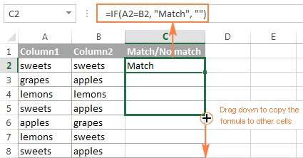
If your objective is to pinpoint rows where column A and column B have identical entries, the following IF formula is your solution. In cell C2, enter:
=IF(A2=B2,"Match","")
This formula operates as follows: It checks if the value in cell A2 is equal to the value in cell B2. If they are the same (a “Match”), it displays “Match” in cell C2. If they are different, it leaves cell C2 blank (“”).
To apply this comparison to all rows, simply click on the small square at the bottom-right corner of cell C2 (the fill handle) and drag it down to cover all the rows you wish to compare.
Formula to Find Differences
Conversely, if you need to highlight rows where column A and column B contain different values, you can easily modify the formula by using the “not equal to” operator (<>). In cell C2, enter:
=IF(A2<>B2,"No match","")
This time, the formula checks if the value in A2 is not equal to the value in B2. If they are different (“No match”), it displays “No match” in cell C2. If they are the same, cell C2 remains blank. Again, drag the fill handle down to apply this to all rows.
Combining Matches and Differences in One Formula
For a more comprehensive result, you can create a single formula that indicates both “Match” and “No match” within the same column. Here are two variations:
=IF(A2=B2,"Match","No match")
Or
=IF(A2<>B2,"No match","Match")
The first formula will display “Match” if the values are the same and “No match” if they are different. The second formula reverses this, displaying “No match” for differences and “Match” for identical values.
The output of these formulas will clearly show you which rows have matching or differing values in columns A and B.
It’s important to note that these IF function formulas seamlessly handle various data types, including numbers, dates, times, and text strings. They provide a robust and straightforward way to compare two columns for matches and differences on a row-by-row basis.
Example 2: Case-Sensitive Comparison for Exact Matches
By default, Excel formulas like the ones above perform case-insensitive comparisons when dealing with text. This means “Apple” and “apple” would be considered a match. However, in scenarios where case sensitivity is critical, Excel offers the EXACT function.
The EXACT function compares two text strings and returns TRUE if they are exactly the same, including case, and FALSE otherwise. To perform a case-sensitive comparison for matches, use the following formula in cell C2:
=IF(EXACT(A2, B2), "Match", "")
This formula uses EXACT(A2, B2) as the logical test within the IF function. If the EXACT function returns TRUE (meaning an exact, case-sensitive match), the formula displays “Match”. Otherwise, it displays nothing.
For case-sensitive differences, you can adapt the formula to:
=IF(EXACT(A2, B2), "Match", "Unique")
In this case, if EXACT returns FALSE (case-sensitive difference), the formula displays “Unique”.
Comparing Multiple Columns for Matches within a Row
Excel also enables you to compare more than two columns within the same row to find matches based on different criteria. Let’s explore how to find matches across multiple columns.
Example 1: Finding Rows with Matches in All Cells
Imagine you have a table with several columns, and you want to identify rows where all cells across those columns contain the same value. For instance, you might have columns A, B, and C, and you want to find rows where A2=B2 and A2=C2 (and therefore B2=C2 as well).
For a small number of columns, you can use the AND function within an IF formula. For three columns (A, B, C), the formula in cell D2 would be:
=IF(AND(A2=B2, A2=C2), "Full match", "")
This formula uses AND(A2=B2, A2=C2) to check if both conditions (A2=B2 and A2=C2) are TRUE. Only if both are true, indicating a “Full match” across all three columns, will “Full match” be displayed.
However, for tables with many columns, using AND can become cumbersome. A more efficient and scalable approach is to use the COUNTIF function. Assuming you are comparing columns A to E (5 columns), the formula in cell F2 would be:
=IF(COUNTIF($A2:$E2, $A2)=5, "Full match", "")
Here’s how this COUNTIF formula works: COUNTIF($A2:$E2, $A2) counts how many cells within the range A2:E2 are equal to the value in cell A2. If all 5 cells in the range are identical to A2 (meaning they are all the same), COUNTIF will return 5. The formula then checks if this count equals 5. If it does, it signifies a “Full match” across all columns.
Example 2: Finding Rows with Matches in Any Two Cells
In other scenarios, you might want to find rows where at least two cells within a row have matching values, regardless of which columns they are in. For example, in columns A, B, and C, you’d want to identify rows where A2=B2, or B2=C2, or A2=C2.
For a smaller number of columns, you can use the OR function in conjunction with IF. For three columns (A, B, C), the formula in cell D2 would be:
=IF(OR(A2=B2, B2=C2, A2=C2), "Match", "")
The OR(A2=B2, B2=C2, A2=C2) part checks if any of the three conditions are TRUE. If at least one condition is true, indicating a match between any two cells in the row, the formula displays “Match”.
When dealing with a larger number of columns, an OR statement can become lengthy and harder to manage. A more concise alternative involves using multiple COUNTIF functions and summing their results. For example, to check for matches among columns A, B, C, and D, you could use:
=IF(COUNTIF(B2:D2,A2)+COUNTIF(C2:D2,B2)+(C2=D2)=0,"Unique","Match")
This formula cleverly combines COUNTIF and direct comparison to identify matches between any two cells within the row across columns A, B, C, and D. If the sum of the COUNTIF results and the direct comparison equals 0, it means no matches were found, and it returns “Unique”; otherwise, it returns “Match”.
Comparing Two Columns for Matches and Differences (List Comparison)
Often, you’ll have two separate lists of data in different columns, and you need to determine which values from the first list are present (or absent) in the second list. This is a common task in data cleaning and reconciliation.
For this type of comparison, the COUNTIF function is particularly effective. Let’s assume your first list is in column A and your second list is in column B. To find values in column A that are not present in column B, you can use the following formula in cell C2 (and drag it down):
=IF(COUNTIF($B:$B, $A2)=0, "No match in B", "")
Let’s break down this formula: COUNTIF($B:$B, $A2) counts how many times the value in cell A2 appears within the entire column B ($B:$B). The $ signs before the column letter ‘B’ ensure that the column B range remains fixed when you drag the formula down. If COUNTIF returns 0, it means the value from A2 is not found anywhere in column B. In this case, the IF function displays “No match in B”. If COUNTIF returns a number greater than 0, it indicates a match is found in column B, and the formula displays an empty string (“”).
For improved performance with very large datasets, instead of referencing the entire column $B:$B, you can specify a more limited range, such as $B$2:$B$1000, if you know the approximate extent of your second list.
Alternatively, you can achieve the same result using a combination of ISERROR and MATCH functions:
=IF(ISERROR(MATCH($A2,$B$2:$B$10,0)),"No match in B","")
The MATCH($A2,$B$2:$B$10,0) function attempts to find the position of the value in A2 within the range B2:B10. If a match is found, MATCH returns the position number; otherwise, it returns an error (#N/A). The ISERROR function checks if MATCH returns an error. If it does (meaning no match), ISERROR returns TRUE, and the IF function displays “No match in B”.
Another approach involves using an array formula with SUM and double negation (--):
=IF(SUM(--($B$2:$B$10=$A2))=0, " No match in B", "")
Remember to enter this array formula by pressing Ctrl + Shift + Enter. The ($B$2:$B$10=$A2) part creates an array of TRUE and FALSE values by comparing A2 to each cell in B2:B10. The double negation (--) converts TRUE to 1 and FALSE to 0. SUM then adds up these 1s and 0s. If the sum is 0, it means no matches were found, and the formula displays “No match in B”.
To identify both matches and differences in a single formula, you can modify any of the above formulas to display a different text string for matches. For example, using COUNTIF:
=IF(COUNTIF($B:$B, $A2)=0, "No match in B", "Match in B")
This version will display “No match in B” for unique values in column A and “Match in B” for values that are also present in column B.
Pulling Matching Data from Two Lists
Beyond simply identifying matches, you might need to retrieve associated data from the second list when a match is found. Excel offers powerful lookup functions for this purpose: VLOOKUP, INDEX MATCH, and XLOOKUP.
For instance, imagine you have a list of product IDs in column D and a master product list with IDs in column A and corresponding sales figures in column B. You want to compare column D’s product IDs against column A and, if a match is found, pull the sales figure from column B.
Here are formulas using each of the lookup functions to achieve this, placed in cell E2 and dragged down:
VLOOKUP:
=VLOOKUP(D2, $A$2:$B$6, 2, FALSE)
INDEX MATCH:
=INDEX($B$2:$B$6, MATCH($D2, $A$2:$A$6, 0))
XLOOKUP (Excel 2021 and Microsoft 365):
=XLOOKUP(D2, $A$2:$A$6, $B$2:$B$6)
Each of these formulas compares the product ID in D2 with the product IDs in the range A2:A6. If a match is found, they retrieve the corresponding sales figure from column B (or the range B2:B6). If no match is found, they typically return an #N/A error.
For a more detailed explanation of VLOOKUP in column comparison, refer to dedicated resources on “How to compare two columns using VLOOKUP”.
Highlighting Matches and Differences Visually with Conditional Formatting
Excel’s Conditional Formatting feature provides a visually intuitive way to highlight matches and differences when comparing columns. You can apply formatting rules to automatically shade cells based on comparison results, making patterns and discrepancies immediately apparent.
Example 1: Highlighting Row-by-Row Matches and Differences
To highlight cells in column A that have the same value as their corresponding cells in column B within the same row, follow these steps:
- Select the cells in column A that you want to format (e.g., A2:A10).
- Go to Home tab > Conditional Formatting > New Rule.
- Choose “Use a formula to determine which cells to format”.
- In the “Format values where this formula is true” box, enter the formula:
=$B2=$A2(Ensure you use a relative row reference for column A, like$A2). - Click the Format button, choose your desired formatting (e.g., fill color), and click OK twice.
To highlight differences instead, repeat the steps but use the formula: =$B2<>$A2
Example 2: Highlighting Unique Entries in Each List
To highlight values that are present in only one of the two lists (unique values), you can use COUNTIF within conditional formatting rules. Assume List 1 is in A2:A6 and List 2 is in C2:C5.
To highlight unique values in List 1 (column A):
- Select cells A2:A6.
- Create a new conditional formatting rule using the formula:
=COUNTIF($C$2:$C$5, $A2)=0 - Choose your formatting.
To highlight unique values in List 2 (column C):
- Select cells C2:C5.
- Create a new rule with the formula:
=COUNTIF($A$2:$A$6, $C2)=0 - Choose formatting.
Example 3: Highlighting Matches (Duplicates) Between Two Columns
To highlight values that are present in both lists (duplicates or matches), adjust the COUNTIF formulas in the conditional formatting rules.
To highlight matches in List 1 (column A):
- Select cells A2:A6.
- Create a new rule with the formula:
=COUNTIF($C$2:$C$5, $A2)>0 - Choose formatting.
To highlight matches in List 2 (column C):
- Select cells C2:C5.
- Create a new rule with the formula:
=COUNTIF($A$2:$A$6, $C2)>0 - Choose formatting.
Highlighting Row Differences and Matches in Multiple Columns
When comparing multiple columns row-by-row, conditional formatting and Excel’s “Go To Special” feature offer efficient ways to visualize matches and differences.
Example 1: Highlighting Rows with Matches Across Multiple Columns
To highlight entire rows where all compared columns have identical values, use conditional formatting with formulas like:
=AND($A2=$B2, $A2=$C2) (for columns A, B, C)
or
=COUNTIF($A2:$C2, $A2)=3 (for 3 columns)
- Select the rows you want to format.
- Create a new conditional formatting rule using one of these formulas.
- Choose your formatting.
Example 2: Highlighting Row Differences in Multiple Columns using “Go To Special”
For quickly highlighting cells with different values within each row compared to a “comparison column,” use Excel’s “Go To Special” feature:
- Select the range of columns you want to compare (e.g., A2:C8). The topmost cell in the selection becomes the active cell and the “comparison column.”
- Go to Home tab > Find & Select > Go To Special.
- Choose “Row differences” and click OK.
- Cells with values different from the comparison cell in each row will be selected.
- Apply a fill color using the Fill Color icon on the ribbon.
Comparing Two Individual Cells
Comparing two individual cells is a simplified instance of row-by-row column comparison. You can directly use IF formulas without needing to drag them down.
To compare cells A1 and C1 for matches:
=IF(A1=C1, "Match", "")
For differences:
=IF(A1<>C1, "Difference", "")
Formula-Free Column Comparison using Add-ins
For users seeking formula-free solutions, Excel add-ins like Ablebits’ “Compare Two Tables” offer a user-friendly interface for comparing columns and lists. These add-ins often provide advanced features and streamlined workflows for identifying matches and differences, highlighting results, and generating reports. While this article primarily focuses on Excel’s built-in capabilities, add-ins can be valuable tools for users who prefer visual interfaces and enhanced functionality.
In Conclusion
Excel provides a rich toolkit for effectively comparing two columns for matches and differences. From basic IF formulas to advanced COUNTIF, MATCH, lookup functions, and conditional formatting, you have numerous options to suit various comparison needs. Whether you’re a beginner or an experienced Excel user, mastering these techniques will significantly enhance your data analysis efficiency and accuracy. By choosing the appropriate method based on your specific requirements, you can confidently tackle column comparison tasks and unlock valuable insights from your data.