In the realm of quantitative image analysis, particularly within fluorescence microscopy, accurately assessing the degree of colocalization between different probes is crucial. This article, brought to you by COMPARE.EDU.VN, delves into the challenges and complexities surrounding the comparison of Pearson’s Correlation Coefficient (PCC) with block values when analyzing colocalization data. Understanding these nuances is essential for researchers aiming to derive meaningful insights from their experimental results. We offer a detailed breakdown, optimized for search engines, to illuminate the intricacies involved.
1. Introduction: The Significance of Colocalization Analysis
Colocalization analysis, a cornerstone of modern cell biology, allows researchers to determine the extent to which two or more distinct molecules reside within the same cellular compartments. This method has applications including verifying molecular interactions and mapping intracellular activity. COMPARE.EDU.VN recognizes the need for clear, concise, and effective methods. Yet, the difficulty lies in the nuances. This review explores the significance of PCC and fractional overlap, including MCC. Effective analysis of co-occurrence is the overall objective.
2. Understanding Pearson’s Correlation Coefficient (PCC) in Colocalization
PCC, developed by Karl Pearson, helps measure the linear relationship between two sets of variables. PCC quantifies how well data points fit a linear pattern. A value of +1 indicates a perfect positive correlation, -1 a perfect negative correlation, and 0 no linear correlation. In biological research, the distribution is measured in images.
2.1. The Formula and Its Implications
The formula for PCC, given two channels (red and green), is:
PCC = ∑i(Ri−R¯)×(Gi−G¯) / √∑i(Ri−R¯)2×∑i(Gi−G¯)2
where *Ri and Gi refer to the intensity values of the red and green channels, respectively, of pixel i, and R̄ and Ḡ* refer to the mean intensities of the red and green channels, respectively, across the entire image.
This means PCC measures the covariance between the signals, subtracting the mean from each pixel. Thus, PCC is independent from signal levels.
2.2. Advantages of Using PCC
One of the reasons to measure PCC when analyzing colocalization is its simplicity. Since PCC measures the covariance between the signal intensity levels of two images on a pixel-by-pixel level, it is often employed in biological microscopy. Furthermore, PCC has tools which are provided in almost all imaging software.
2.3. Limitations of PCC in Colocalization Studies
The meaning of extreme PCC values is clear but interpretation of intermediate values is more complex.
PCC also measures the degree to which a linear relationship can be determined, providing a weak measure of colocalization in complex situations, e.g. when probes co-occur in different proportions across different cell compartments. If data is more complex than a simple linear regression, it is ambiguous, if not misleading.
3. Exploring Block Values and Their Role in Spatial Analysis
Block values, in the context of image analysis, refer to the aggregation of pixel data within defined blocks or regions. This approach is particularly relevant when addressing spatial autocorrelation, where the value of one pixel is influenced by the values of its neighboring pixels.
3.1. Addressing Spatial Autocorrelation
One challenge of PCC is that the sample may have auto-correlation. Essentially, after developing PCC, it was demonstrated that autocorrelation can yield statistically significant correlations, even for variables with no real association. Low-pass filtering can increase autocorrelation, and aggravate spatial filters used to reduce image noise.
3.2. The Significance of Block Size
Block sizes must be equal to or exceed the size of objects in an image. Fragmentation of the original image decreases auto-correlation. Autocorrelation also affects significance testing of MCC.
3.3. Applying Block Scrambling Techniques
The pixel block scrambling approach is used to estimate a measurement’s random probability, and has been implemented in Slidebook software and the JACoP and WCIF ImageJ plugins. This has a capability to adjust the block size used for randomization. In these analyses, an image is generated where a white noise image is convolved with a Gaussian filter that matches that of the imaging system. This will be appropriate when analyzing the structure’s images when the images are similar in size.
4. The Central Question: Why “Could Not Compare Pearson With Block Values”?
The error message “Could Not Compare Pearson With Block Values” typically arises due to fundamental incompatibilities between these analytical approaches. PCC is a pixel-based correlation metric, while block values involve aggregated data. COMPARE.EDU.VN identifies key scenarios where this issue manifests:
4.1. Data Type Mismatch
PCC is calculated using the intensity values of individual pixels, while block values represent aggregated data (e.g., the mean intensity of a block of pixels). These are fundamentally different data types, and attempting to directly compare them is statistically unsound.
4.2. Scale of Analysis Differences
PCC operates at the level of individual pixels, capturing fine-grained correlations. Block values, on the other hand, provide a coarser, more regional perspective. Direct comparison can obscure important details and lead to misinterpretations.
4.3. Statistical Assumptions Violation
Statistical tests rely on specific assumptions about the data. Comparing PCC and block values may violate these assumptions, leading to invalid statistical conclusions. PCC and block values are often not interchangeable when analyzing the data.
5. Alternative Methodologies for Colocalization Analysis
When direct comparison of PCC with block values is not feasible, COMPARE.EDU.VN recommends exploring alternative methodologies:
5.1. Manders’ Colocalization Coefficients (MCC)
MCC provides a measure of colocalization that is more intuitive, namely, the fraction of each probe that is colocalized with the other. Because MCC can measure two probes independently, it does not depend on a relationship. MCC measurements are sensitive to the background level, so each sample must be evaluated consistently.
5.2. Object-Based Colocalization Analysis
This approach involves identifying and segmenting individual objects (e.g., vesicles, organelles) within the images and then quantifying their spatial relationships. Object-based measures, such as the percentage of objects that overlap or the distance between objects, can provide valuable insights into colocalization patterns. It is appropriate for integral membrane proteins or the distribution of nuclear proteins.
5.3. Intensity Correlation Analysis
Instead of relying solely on PCC, consider using intensity correlation analysis to identify regions of high or low correlation between the two channels. This can provide a more nuanced view of colocalization, particularly in cases where the relationship between the probes is not strictly linear.
6. Practical Strategies for Resolving the Comparison Issue
To address the issue of “Could Not Compare Pearson With Block Values,” consider the following practical strategies:
6.1. Aligning the Scales of Analysis
If the goal is to relate PCC to regional data, calculate PCC within each block and then analyze the distribution of PCC values across the blocks.
6.2. Transforming Block Values
Transform block values into a pixel-level representation by assigning the block value to each pixel within the block. Then, calculate PCC using these pixel-level representations. Be cautious, as this inflates autocorrelation.
6.3. Statistical Considerations
Consult with a statistician to determine appropriate statistical tests for comparing PCC and block values, taking into account the data structure and potential violations of statistical assumptions.
7. Case Studies and Examples
Let’s consider a few case studies where the “Could Not Compare Pearson With Block Values” issue might arise and how to address it:
7.1. Case Study 1: Analyzing Protein Colocalization in Endosomes
In this scenario, we want to determine whether two proteins, A and B, colocalize within endosomes.
- Challenge: We have PCC values for individual cells and block values representing the average expression level of protein B in different regions of the cell.
- Solution: Instead of directly comparing PCC and block values, calculate PCC within each block and then correlate the mean PCC with the average expression level of protein B in that block.
7.2. Case Study 2: Investigating Colocalization of Synaptic Proteins
Here, we aim to assess the colocalization of two synaptic proteins, X and Y, at the synapse.
- Challenge: We have PCC values for individual synapses and block values representing the density of synapses in different brain regions.
- Solution: Calculate the average PCC for all synapses within each brain region and then compare the average PCC with the synapse density.
8. Advanced Techniques for Enhanced Colocalization Analysis
To further enhance colocalization analysis and avoid the “Could Not Compare Pearson With Block Values” issue, consider these advanced techniques:
8.1. Super-Resolution Microscopy
Super-resolution microscopy techniques, such as stimulated emission depletion (STED) microscopy and structured illumination microscopy (SIM), offer improved spatial resolution, enabling more precise colocalization analysis.
8.2. Machine Learning Approaches
Machine learning algorithms can be trained to automatically identify and quantify colocalization patterns in complex images, reducing user bias and improving accuracy.
8.3. Bayesian Inference
Bayesian inference provides a statistical framework for incorporating prior knowledge into colocalization analysis, improving the reliability of the results.
9. Validating Your Colocalization Analysis: Essential Controls
Regardless of the method used, validation is paramount. This includes:
- Positive Controls: Use known interacting molecules to confirm colocalization detection.
- Negative Controls: Use non-interacting molecules to rule out false positives.
- Randomization Techniques: Scramble images to test significance against random overlap.
10. Best Practices for Colocalization Studies
To ensure reliable and reproducible colocalization results, COMPARE.EDU.VN recommends adhering to these best practices:
10.1. Optimize Image Acquisition
Carefully optimize image acquisition parameters to minimize noise and background and maximize signal-to-noise ratio.
10.2. Use Appropriate Controls
Include appropriate positive and negative controls to validate the colocalization analysis and rule out artifacts.
10.3. Report Methodology Clearly
Thoroughly document the image analysis methodology, including software, parameters, and statistical tests used.
10.4. Consider Biological Context
Interpret colocalization results in the context of the biological system being studied, taking into account known interactions and regulatory mechanisms.
10.5. Implement Proper Image Collection
The first step is the design and image collection. Probes should be sensitive and specific, ideally determined in control studies. Collect fluorescence signals in a linear range. Crosstalk between signals between channels should be negligible. Images of the entire three-dimensional volume should be acquired, since it is better to collect volumetric data than to repeat a study.
10.6. Identify Question to be Answered
Before determining the next step, determine if quantification is necessary. Quantification is most useful when comparisons are being made between different conditions. In addition, some instances are visually obvious.
10.7. Decide Which Metric to Use
The choice for most studies is between a form of PCC and MCC. One should not be considered superior to the other, the biological question should inform the selection. Data should first be evaluated for linearity. Randomly identify cells to be quantified. Compare values measured from single planes to the entire volume to determine whether PCC in the volumes is warranted.
10.8. Follow a Careful Plan
One should then identify cells to be quantified and outline the relevant ROI for each. Then, compare the values from each plane with those obtained from the entire volume to determine if volume measurement of PCC is warranted.
11. Overcoming Challenges: Troubleshooting Common Issues
Colocalization analysis can be fraught with challenges. Here’s how to troubleshoot common issues:
11.1. High Background Noise
Optimize image acquisition parameters and use background subtraction techniques to reduce noise.
11.2. Bleed-Through Between Channels
Carefully select fluorophores and use spectral unmixing techniques to minimize bleed-through.
11.3. Incomplete or Uneven Labeling
Optimize labeling protocols and use image restoration techniques to correct for uneven labeling.
11.4. Object Segmentation Errors
Fine-tune object segmentation parameters and use manual correction to improve accuracy.
12. Future Directions in Colocalization Analysis
The field of colocalization analysis is constantly evolving. Here are some potential future directions:
12.1. Integration with Multi-Omics Data
Combining colocalization data with other omics data (e.g., genomics, proteomics) can provide a more holistic understanding of cellular processes.
12.2. Development of More Robust Algorithms
Researchers are working to develop more robust algorithms that are less sensitive to noise and artifacts and can handle complex colocalization patterns.
12.3. Real-Time Colocalization Analysis
Advances in microscopy and image analysis techniques are enabling real-time colocalization analysis, providing insights into dynamic cellular processes.
13. COMPARE.EDU.VN: Your Partner in Colocalization Analysis
COMPARE.EDU.VN is committed to providing researchers with the resources and information they need to conduct successful colocalization studies. Contact us today to learn more about our services and how we can help you achieve your research goals.
Address: 333 Comparison Plaza, Choice City, CA 90210, United States
Whatsapp: +1 (626) 555-9090
Website: COMPARE.EDU.VN
14. Conclusion: Navigating the Complexities of Colocalization Analysis
Colocalization analysis, while powerful, requires careful consideration of the underlying principles and potential pitfalls. The “Could Not Compare Pearson With Block Values” error highlights the importance of understanding the limitations of different analytical approaches and selecting appropriate methodologies for each specific research question. By adhering to best practices, validating results, and staying abreast of new developments, researchers can unlock the full potential of colocalization analysis and gain valuable insights into the complexities of cellular function.
15. Frequently Asked Questions (FAQ)
Here are some frequently asked questions about colocalization analysis:
-
What is colocalization analysis?
Colocalization analysis is a technique used to determine the extent to which two or more distinct molecules reside within the same cellular compartments.
-
What is Pearson’s Correlation Coefficient (PCC)?
PCC is a statistical measure of the linear correlation between two variables. In colocalization analysis, it quantifies the correlation between the intensity values of two channels in an image.
-
What are block values?
Block values refer to the aggregation of pixel data within defined blocks or regions of an image.
-
Why can’t I directly compare Pearson with block values?
Direct comparison is statistically unsound due to data type mismatches, scale of analysis differences, and potential violations of statistical assumptions.
-
What are some alternative methodologies for colocalization analysis?
Alternatives include Manders’ Colocalization Coefficients (MCC), object-based colocalization analysis, and intensity correlation analysis.
-
What are some practical strategies for resolving the comparison issue?
Strategies include aligning the scales of analysis, transforming block values, and consulting with a statistician.
-
What are some best practices for colocalization studies?
Best practices include optimizing image acquisition, using appropriate controls, reporting methodology clearly, and considering biological context.
-
How can I validate my colocalization analysis?
Validation involves using positive and negative controls and randomization techniques.
-
What are some common challenges in colocalization analysis?
Challenges include high background noise, bleed-through between channels, incomplete or uneven labeling, and object segmentation errors.
-
What are some future directions in colocalization analysis?
Future directions include integration with multi-omics data, development of more robust algorithms, and real-time colocalization analysis.
By addressing these FAQs and implementing the strategies outlined in this article, researchers can overcome the challenges of colocalization analysis and obtain reliable, reproducible results. Visit COMPARE.EDU.VN for more information and resources.
This image shows a maximum projection of Madin Darby Canine Kidney cells following incubation with Texas Red and Alexa 488, indicating endosomes containing both probes for colocalization analysis.
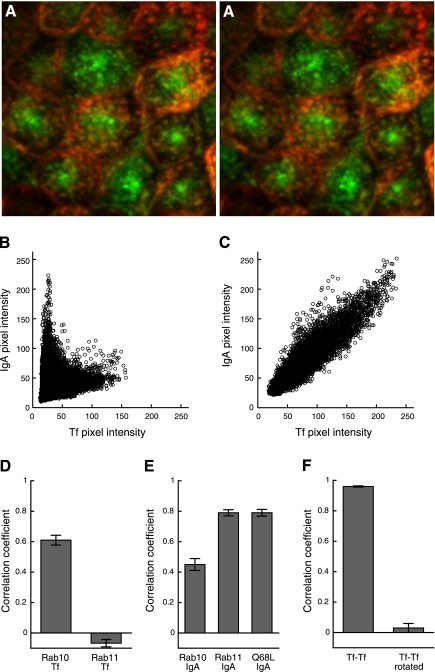
This image demonstrates colocalization analysis of endocytic probes with scatterplots of red and green pixel intensities showing internalized IgA and transferrin in MDCK cells with and without brefeldinA treatment.
This graphic illustrates the importance of the region of interest (ROI) for measuring Pearson’s Correlation Coefficient (PCC) using transfected Chinese hamster ovary (CHO) cells incubated with Texas Red-transferrin and Oregon Green-IgA.
This focal plane shows an MDCK cell illustrating colocalization without a simple linear relationship, with cells incubated with Texas Red-transferrin and Oregon Green IgA and scatterplots of red and green pixel intensities.
This image illustrates Manders’ Overlap Coefficient (MOC) as a measure of colocalization using scatterplots showing positively, negatively, and uncorrelated red and green pixel values and measurements for uncorrelated data as a function of offset.
This image illustrates the Costes automatic thresholding method in colocalization analysis, showing single image planes of MDCK cells and binary versions of the images after applying Costes thresholds.
This composite shows background correction using the Costes automatic thresholding method and median subtraction techniques applied to image volumes and single planes of MDCK and CHO cells.
This schematic outlines a general colocalization analysis workflow starting from validating fluorescent probes to quantifying PCC or MCC after imaging and applying designated ROIs.
This image shows significance testing of colocalization data with scatterplots of pixel values and distributions of MCC values obtained after randomly distributing or scrambling pixel segments.
Ready to make smarter comparisons? Visit compare.edu.vn today and discover the best choices for your needs.