Comparing Two Columns in Excel to Find Differences

Comparing Two Columns In Excel To Find Differences is a common task for data analysis, cleaning, and validation. Whether you’re reconciling financial records, comparing customer lists, or identifying discrepancies in inventory, Excel provides several methods to efficiently pinpoint those variations. COMPARE.EDU.VN empowers you with the knowledge and tools to effectively compare data, identify discrepancies, and make informed decisions. Master techniques like IF functions, conditional formatting, and specialized tools for streamlined data comparison.

1. Understanding the Need for Comparing Columns in Excel

Before diving into the methods, it’s crucial to understand why comparing two columns in Excel is essential. Data discrepancies can arise from various sources, including manual data entry errors, inconsistencies in data formats, or updates that haven’t been synchronized across different datasets. Identifying these differences is critical for maintaining data accuracy, ensuring data integrity, and making informed decisions based on reliable information. Let’s explore the key reasons for comparing columns:

Data Validation: Ensure the accuracy and consistency of data by identifying discrepancies between two sets of data.
Error Detection: Locate and correct errors in data entry, calculations, or data transfers.
Data Reconciliation: Compare data from different sources to identify and resolve inconsistencies.
Change Tracking: Monitor changes made to data over time by comparing previous and current versions.
Data Integration: Verify the accuracy of data when merging data from multiple sources.
List Management: Identify unique or duplicate entries in lists.
Auditing: Ensure data accuracy and compliance with regulations.
Reporting: Generate reports that highlight differences between data sets.
Decision Making: Make informed decisions based on accurate and reliable data.
Process Improvement: Identify areas where data entry or data management processes can be improved.

2. Essential Excel Functions for Column Comparison

Excel offers a range of built-in functions that can be used to compare columns effectively. These functions can help you identify matches, differences, and unique values. Below are some essential Excel functions for this purpose:

IF Function: This function allows you to perform logical tests and return different values based on the outcome. It is useful for identifying matches and differences between individual cells in two columns.
COUNTIF Function: This function counts the number of cells within a range that meet a specific criterion. It can be used to determine whether a value in one column exists in another column.
EXACT Function: This function compares two text strings and returns TRUE if they are exactly the same (case-sensitive) and FALSE otherwise. It is useful for case-sensitive comparisons.
MATCH Function: This function searches for a specified item in a range of cells and returns the relative position of that item in the range. It can be used to determine if a value in one column exists in another column and to find its location.
ISERROR Function: This function checks whether a formula results in an error and returns TRUE if it does, and FALSE otherwise. It can be used in conjunction with the MATCH function to handle errors when a value is not found.
VLOOKUP Function: This function searches for a value in the first column of a table and returns a value in the same row from another column in the table. It can be used to compare two columns and retrieve associated data from one column based on a match in the other.
INDEX and MATCH Functions: These functions can be used together to perform more flexible lookups than VLOOKUP. INDEX returns the value of a cell in a table based on the row and column numbers, while MATCH finds the position of a value in a range.
XLOOKUP Function: This function is a more modern and versatile lookup function that replaces VLOOKUP, HLOOKUP, and INDEX/MATCH. It can search for a value in a range and return a corresponding value from another range, with options for handling errors and specifying match types.

3. Comparing Two Columns Row by Row Using the IF Function

One of the simplest methods for comparing two columns in Excel is to use the IF function. This method allows you to compare corresponding cells in two columns and determine if they match or differ.

3.1. Formula for Matches

To find cells within the same row having the same content, for example, A2 and B2, the formula is as follows:

=IF(A2=B2,"Match","")

This formula compares the values in cells A2 and B2. If the values are equal, the formula returns “Match”; otherwise, it returns an empty string (“”).

3.2. Formula for Differences

To find cells in the same row with different values, simply replace the equals sign (=) with the non-equality sign (<>):

=IF(A2<>B2,"No match","")

This formula compares the values in cells A2 and B2. If the values are different, the formula returns “No match”; otherwise, it returns an empty string (“”).

3.3. Matches and Differences

And of course, nothing prevents you from finding both matches and differences with a single formula:

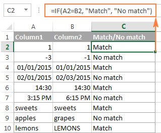
=IF(A2=B2,"Match","No match")

=IF(A2<>B2,"No match","Match")

The result may look similar to this.

As you see, the formula handles numbers, dates, times, and text strings equally well.

Tip: You can also compare two columns row-by-row using Excel Advanced Filter. Here is an example showing how to filter matches and differences between 2 columns.

3.4. Case-Sensitive Comparisons

As you have probably noticed, the formulas from the previous example ignore case when comparing text values, as in row 10 in the screenshot above. If you want to find case-sensitive matches between 2 columns in each row, then use the EXACT function:

=IF(EXACT(A2, B2), "Match", "")

To find case-sensitive differences in the same row, enter the corresponding text (“Unique” in this example) in the 3rd argument of the IF function, e.g.:

=IF(EXACT(A2, B2), "Match", "Unique")

4. Comparing Multiple Columns for Matches

In some cases, you may need to compare more than two columns to identify matches or differences. Excel provides formulas that can handle multiple column comparisons.

4.1. Find Matches in All Cells Within the Same Row

If your table has three or more columns and you want to find rows that have the same values in all cells, an IF formula with an AND statement will work a treat:

=IF(AND(A2=B2, A2=C2), "Full match", "")

If your table has a lot of columns, a more elegant solution would be using the COUNTIF function:

=IF(COUNTIF($A2:$E2, $A2)=5, "Full match", "")

Where 5 is the number of columns you are comparing.

4.2. Find Matches in Any Two Cells in the Same Row

If you are looking for a way to compare columns for any two or more cells with the same values within the same row, use an IF formula with an OR statement:

=IF(OR(A2=B2, B2=C2, A2=C2), "Match", "")

In case there are many columns to compare, your OR statement may grow too big in size. In this case, a better solution would be adding up several COUNTIF functions. The first COUNTIF counts how many columns have the same value as in the 1st column, the second COUNTIF counts how many of the remaining columns are equal to the 2nd column, and so on. If the count is 0, the formula returns “Unique”, “Match” otherwise. For example:

=IF(COUNTIF(B2:D2,A2)+COUNTIF(C2:D2,B2)+(C2=D2)=0,"Unique","Match")

5. Using Conditional Formatting to Highlight Differences

Conditional formatting allows you to visually highlight cells based on specific criteria. This can be a powerful way to quickly identify differences between two columns.

5.1. Highlight Matches and Differences in Each Row

To compare two columns and Excel and highlight cells in column A that have identical entries in column B in the same row, do the following:

Select the cells you want to highlight (you can select cells within one column or in several columns if you want to color entire rows).
Click Conditional formatting > New Rule… > Use a formula to determine which cells to format.
Create a rule with a simple formula like =$B2=$A2 (assuming that row 2 is the first row with data, not including the column header). Please double-check that you use a relative row reference (without the $ sign) like in the formula above.

To highlight differences between column A and B, create a rule with this formula:

=$B2<>$A2

If you are new to Excel conditional formatting, please see How to create a formula-based conditional formatting rule for step-by-step instructions.

5.2. Highlight Unique Entries in Each List

Whenever you are comparing two lists in Excel, there are 3 item types that you can highlight:

Items that are only in the 1st list (unique)
Items that are only in the 2nd list (unique)
Items that are in both lists (duplicates) – demonstrated in the next example.

This example demonstrates how to color the items that are only in one list.

Supposing your List 1 is in column A (A2:A6) and List 2 in column C (C2:C5). You create the conditional formatting rules with the following formulas:

Highlight unique values in List 1 (column A):

=COUNTIF($C$2:$C$5, $A2)=0

Highlight unique values in List 2 (column C):

=COUNTIF($A$2:$A$6, $C2)=0

And get the following result:

5.3. Highlight Matches (Duplicates) Between 2 Columns

If you closely followed the previous example, you won’t have difficulties adjusting the COUNTIF formulas so that they find the matches rather than differences. All you have to do is to set the count greater than zero:

Highlight matches in List 1 (column A):

=COUNTIF($C$2:$C$5, $A2)>0

Highlight matches in List 2 (column C):

=COUNTIF($A$2:$A$6, $C2)>0

6. Comparing Two Lists for Matches and Differences

Suppose you have 2 lists of data in Excel, and you want to find all values (numbers, dates or text strings) which are in column A but not in column B.

For this, you can embed the COUNTIF($B:$B, $A2)=0 function in IF’s logical test and check if it returns zero (no match is found) or any other number (at least 1 match is found).

For instance, the following IF/COUNTIF formula searches across the entire column B for the value in cell A2. If no match is found, the formula returns “No match in B”, an empty string otherwise:

=IF(COUNTIF($B:$B, $A2)=0, "No match in B", "")

Tip: If your table has a fixed number of rows, you can specify a certain range (e.g. $B2:$B10) rather than the entire column ($B:$B) for the formula to work faster on large data sets.

The same result can be achieved by using an IF formula with the embedded ISERROR and MATCH functions:

=IF(ISERROR(MATCH($A2,$B$2:$B$10,0)),"No match in B","")

Or, by using the following array formula (remember to press Ctrl + Shift + Enter to enter it correctly):

=IF(SUM(--($B$2:$B$10=$A2))=0, " No match in B", "")

If you want a single formula to identify both matches (duplicates) and differences (unique values), put some text for matches in the empty double quotes (“”) in any of the above formulas. For example:

=IF(COUNTIF($B:$B, $A2)=0, "No match in B", "Match in B")

7. How to Compare Two Lists in Excel and Pull Matches

Sometimes you may need not only match two columns in two different tables, but also pull matching entries from the lookup table. Microsoft Excel provides a special function for this – the VLOOKUP function. As an alternative, you can use a more powerful and versatile INDEX MATCH formula. The users of Excel 2021 and Excel 365 can accomplish the task with the XLOOKUP function.

For example, the following formulas compare the product names in columns D against the names in column A and pull a corresponding sales figure from column B if a match is found, otherwise the #N/A error is returned.

=VLOOKUP(D2, $A$2:$B$6, 2, FALSE)

=INDEX($B$2:$B$6, MATCH($D2, $A$2:$A$6, 0))

=XLOOKUP(D2, $A$2:$A$6, $B$2:$B$6)

For more information, please see How to compare two columns using VLOOKUP.

If you don’t feel very comfortable with formulas, you can have the job done using a fast and intuitive solution – Merge Tables Wizard.

8. Comparing Multiple Columns and Highlighting Row Differences

To quickly highlight cells with different values in each individual row, you can use Excel’s Go To Special feature.

Select the range of cells you want to compare. In this example, I’ve selected cells A2 to C8. By default, the top-most cell of the selected range is the active cell, and the cells from the other selected columns in the same row will be compared to that cell. As you can see in the screenshot above, the active cell is white while all other cells of the selected range are highlighted. In this example, the active cell is A2, so the comparison column is column A.

To change the comparison column, use either the Tab key to navigate through selected cells from left to right, or the Enter key to move from top to bottom.

Tip: To select non-adjacent columns, select the first column, press and hold Ctrl, and then select the other columns. The active cell will be in the last column (or in the last block of adjacent columns). To change the comparison column, use the Tab or Enter key as described above.
On the Home tab, go to Editing group, and click Find & Select > Go To Special… Then select Row differences and click the OK button.

The cells whose values are different from the comparison cell in each row are colored. If you want to shade the highlighted cells in some color, simply click the Fill Color icon on the ribbon and select the color of your choosing.

9. Formula-Free Way to Compare Two Columns in Excel

Now that you know Excel’s offerings for comparing and matching columns, let me show you our own solution for this task. This tool is named Compare Two Tables and it is included in our Ultimate Suite.

The add-in can compare two tables or lists by any number of columns and both identify matches/differences (as we did with formulas) and highlight them (as we did with conditional formatting).

For the purpose of this article, we’ll be comparing the following 2 lists to find common values that are present in both.

To compare two lists, here are the steps you need to follow:

Start with clicking the Compare Tables button on the Ablebits Data tab.
Select the first column/list and click Next. In terms of the add-in, this is your Table 1.

Select the second column/list and click Next. In terms of the add-in, it is your Table 2, and it can reside in the same or different worksheet or even in another workbook.

Choose what kind of data to look for:
- Duplicate values (matches) – the items that exist in both lists.
- Unique values (differences) – the items that are present in list 1 but not in list 2.
Since our aim is to find matches, we select the first option and click Next.

This is the key step where you select the columns for comparison. In our case, the choice is obvious as we are only comparing 2 columns: 2000 Winners against 2021 Winners. In bigger tables, you can select several column pairs to compare by.

In the final step, you choose how to deal with the found items and click Finish. A few different options are available here. For our purposes, these two are most useful:
- Highlight with color – shades matches or differences in the selected color (like Excel conditional formatting does).
- Identify in the Status column – inserts the Status column with the “Duplicate” or “Unique” labels (like IF formulas do).

For this example, I’ve decided to highlight duplicates in the following color:

And in a moment, got the following result:

With the Status column, the result would look as follows:

Tip: If the lists you are comparing are in different worksheets or workbooks, it might be helpful to view Excel sheets side by side.

10. Best Practices for Comparing Columns in Excel

To ensure accuracy and efficiency when comparing columns in Excel, consider the following best practices:

Data Cleaning: Before comparing data, clean it by removing any leading or trailing spaces, standardizing date formats, and correcting any inconsistencies in text capitalization.
Data Sorting: Sort the data in both columns before comparing them. This can make it easier to identify matches and differences.
Consistent Formulas: Use consistent formulas throughout your worksheet to avoid errors.
Error Handling: Use error handling techniques, such as the IFERROR function, to handle cases where a value is not found.
Testing: Test your formulas and conditional formatting rules on a small sample of data before applying them to the entire dataset.
Documentation: Document your formulas and conditional formatting rules so that others can understand how they work.
Data Validation: Use data validation to ensure that data is entered correctly in the first place.
Backup: Always back up your data before making any changes.
Data Types: Ensure that the data types of the columns you are comparing are the same. For example, if one column contains numbers and the other contains text, you may need to convert the data types before comparing them.
Cell References: Use absolute and relative cell references correctly to ensure that your formulas work as expected when you copy them to other cells.
Auditing: Regularly audit your data to ensure that it remains accurate and consistent.

11. Real-World Applications of Comparing Columns in Excel

Comparing columns in Excel has numerous real-world applications across various industries and domains. Here are a few examples:

Finance: Reconciling bank statements with internal records to identify discrepancies and prevent fraud.
Sales: Comparing sales data from different periods to track performance and identify trends.
Marketing: Comparing customer lists to identify duplicate entries and improve targeting.
Inventory Management: Comparing inventory records with physical counts to identify discrepancies and prevent stockouts.
Human Resources: Comparing employee data to identify inconsistencies and ensure compliance with regulations.
Healthcare: Comparing patient data to identify errors and improve patient care.
Education: Comparing student data to track progress and identify students who need assistance.
Project Management: Comparing project plans with actual progress to identify delays and manage resources.
Manufacturing: Comparing production data to identify inefficiencies and improve quality control.
Retail: Comparing sales data to identify popular products and optimize inventory levels.

12. Frequently Asked Questions (FAQ) About Comparing Two Columns in Excel

Here are some frequently asked questions about comparing two columns in Excel:

Q1: How do I compare two columns in Excel for exact matches?

A1: You can use the EXACT function to compare two columns for case-sensitive matches. For example, =IF(EXACT(A2, B2), "Match", "").

Q2: How can I ignore case when comparing two columns in Excel?

A2: Use the IF function with the equals sign (=) to compare two columns, as it ignores case by default. For example, =IF(A2=B2, "Match", "").

Q3: How do I find unique values in two columns in Excel?

A3: Use the COUNTIF function to determine if a value in one column exists in another column. If the count is 0, the value is unique.

Q4: How can I highlight differences between two columns in Excel?

A4: Use conditional formatting with a formula to highlight cells that have different values. For example, =$A2<>$B2.

Q5: How do I compare two columns and pull matching data from another column?

A5: Use the VLOOKUP, INDEX/MATCH, or XLOOKUP functions to search for a value in one column and retrieve associated data from another column.

Q6: How can I compare multiple columns for matches in Excel?

A6: Use the IF function with the AND statement to find rows that have the same values in all columns. Alternatively, use the COUNTIF function.

Q7: How do I quickly highlight row differences in multiple columns?

A7: Use Excel’s Go To Special feature to select Row differences and then apply a fill color to the highlighted cells.

Q8: How can I compare two lists in Excel and identify duplicates?

A8: Use the COUNTIF function to count the number of times a value in one list appears in the other list. If the count is greater than 0, the value is a duplicate.

Q9: What is the best way to compare two large columns in Excel?

A9: For large datasets, consider using array formulas or Excel add-ins to improve performance.

Q10: Can I compare two columns in Excel if they are in different worksheets?

A10: Yes, you can reference cells in other worksheets by including the worksheet name in the cell reference. For example, =IF(Sheet1!A2=Sheet2!B2, "Match", "").

13. Why Choose COMPARE.EDU.VN for Your Comparison Needs

When it comes to comparing two columns in Excel or any other comparison task, COMPARE.EDU.VN is your trusted resource. We provide comprehensive, objective, and easy-to-understand comparisons across a wide range of categories. Here’s why you should choose COMPARE.EDU.VN:

Comprehensive Comparisons: We provide in-depth comparisons that cover all the key features, specifications, and benefits of different products, services, and ideas.
Objective Information: Our comparisons are based on objective data and analysis, ensuring that you get unbiased information to make informed decisions.
Easy-to-Understand Format: We present our comparisons in a clear and concise format that is easy to understand, even if you are not an expert in the subject matter.
Wide Range of Categories: We cover a wide range of categories, including technology, finance, education, health, and more.
Up-to-Date Information: We keep our comparisons up-to-date with the latest information, so you can be sure that you are getting the most accurate and relevant data.
User Reviews: We include user reviews and ratings to give you a well-rounded perspective on the products and services we compare.
Expert Analysis: Our team of experts provides in-depth analysis and insights to help you understand the pros and cons of each option.
Personalized Recommendations: We offer personalized recommendations based on your specific needs and preferences.
Time-Saving: We save you time by doing the research and analysis for you, so you can focus on making the best decision for your needs.
Free Resource: COMPARE.EDU.VN is a free resource that is available to everyone.

14. Take Action Today

Ready to compare two columns in Excel and find the differences? Visit COMPARE.EDU.VN today to access our comprehensive guides, expert analysis, and user reviews. Make informed decisions and achieve your goals with the help of COMPARE.EDU.VN.

Unlock the power of informed decision-making with COMPARE.EDU.VN. Whether you’re evaluating software, selecting a service, or weighing different ideas, our platform offers the insights you need. Don’t let uncertainty hold you back. Visit COMPARE.EDU.VN now and start comparing! Contact us at 333 Comparison Plaza, Choice City, CA 90210, United States. Whatsapp: +1 (626) 555-9090. Or visit our website: compare.edu.vn.