Comparing Excel Columns for Differences: A Comprehensive Guide

Comparing columns in Excel to identify differences is a crucial skill for data analysis, cleaning, and reporting. Whether you are working with large datasets, reconciling accounts, or simply managing lists, knowing how to pinpoint discrepancies between columns can save you significant time and effort. Microsoft Excel provides a range of built-in features and formulas to accomplish this, from simple row-by-row comparisons to more advanced techniques for highlighting unique entries. This guide will explore various methods for effectively Comparing Excel Columns For Differences, catering to different scenarios and levels of Excel proficiency.

Row-by-Row Comparison for Differences Using Formulas

One of the most fundamental ways to compare columns in Excel is to perform a row-by-row analysis. This approach is particularly useful when you want to see how corresponding entries in two columns differ within each row. Excel’s IF function is perfectly suited for this task, allowing you to flag differences directly.

Identifying Differences in the Same Row with the IF Function

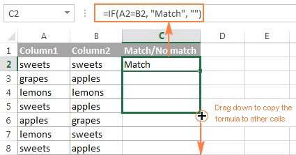
To begin, let’s use the IF function to compare two columns, say column A and column B, and identify rows where the values are different. You’ll insert this formula into a new column (for example, column C) in the first row of your data (assuming your data starts from row 2).

=IF(A2<>B2,"Different","")

In this formula:

A2<>B2 is the comparison. The <> operator means “not equal to.” This checks if the value in cell A2 is different from the value in cell B2.
"Different" is the value that will be displayed if the condition is TRUE (i.e., the values are different).
"" (empty string) is the value that will be displayed if the condition is FALSE (i.e., the values are the same).

After entering this formula in cell C2, you can use the fill handle (the small square at the bottom-right corner of the cell) to drag the formula down to apply it to all rows in your dataset.

This will result in column C highlighting “Different” for every row where column A and column B have differing values.

You can customize the output. For instance, instead of "Different", you could display "Mismatch", "Difference Found", or simply "No" to clearly indicate the rows with discrepancies. You can also modify the empty string "" to display "Match" or "Yes" to explicitly mark rows where the columns are identical if needed.

=IF(A2<>B2,"Mismatch","Match")

This modified formula will now explicitly show both “Mismatch” and “Match” results, giving a clear overview of both types of comparisons.

This method works effectively with numbers, text, dates, and times, making it a versatile approach for various types of data comparison.

Case-Sensitive Difference Checks

By default, Excel’s comparison is not case-sensitive, meaning “Apple” and “apple” are treated as the same. If you need to perform a case-sensitive comparison to find differences, you can use the EXACT function in combination with the IF function. The EXACT function checks if two text strings are exactly the same, including case.

To find case-sensitive differences, use the following formula:

=IF(EXACT(A2,B2),"", "Case Difference")

Here:

EXACT(A2,B2) returns TRUE if A2 and B2 are exactly the same (case-sensitive) and FALSE otherwise.
"" is displayed if EXACT is TRUE (i.e., no case difference).
"Case Difference" is displayed if EXACT is FALSE (i.e., a case difference is found).

This formula will highlight rows where the content is the same except for the case, which can be important in scenarios where case sensitivity matters, such as in password lists or specific identifier columns.

Comparing Lists for Unique Differences

Sometimes, you need to compare two lists of data in separate columns and identify values that are present in one list but not in the other. This is useful for finding unique entries or identifying missing items between lists. The COUNTIF function is excellent for this type of comparison.

Finding Values Unique to One Column

Let’s say you have List 1 in column A and List 2 in column B. To find values in List 1 that are not present in List 2, you can use the following IF and COUNTIF formula in a helper column (e.g., column C):

=IF(COUNTIF($B:$B, A2)=0, "Unique to List 1", "")

In this formula:

COUNTIF($B:$B, A2) counts how many times the value from cell A2 appears in the entire column B ($B:$B). The $ signs make the column B reference absolute, so it doesn’t change when you drag the formula down.
=0 checks if the count is zero, meaning the value from A2 is not found in column B.
"Unique to List 1" is displayed if the count is zero (i.e., the value is unique to List 1).
"" is displayed if the count is greater than zero (i.e., the value is also in List 2).

Similarly, to find values unique to List 2 (column B) that are not in List 1 (column A), you can use a similar formula in another helper column (e.g., column D):

=IF(COUNTIF($A:$A, B2)=0, "Unique to List 2", "")

By using these two formulas, you can effectively identify items that are unique to each list, highlighting the differences between the two columns.

Highlighting Differences Using Conditional Formatting

While formulas are great for programmatically identifying differences, conditional formatting provides a visual approach to highlight these discrepancies directly within your Excel sheet. This method is particularly useful for quickly spotting differences without adding extra columns.

Highlighting Differences in Rows

To highlight cells that are different in each row across two columns (e.g., column A and column B), follow these steps:

Select the range you want to compare (e.g., columns A and B, or just column A if you want to highlight differences in column A based on column B).
Go to Home tab > Conditional Formatting > New Rule.
Select “Use a formula to determine which cells to format”.
Enter the following formula in the “Format values where this formula is true” box:
```
=$A2<>$B2
```
(Assuming row 2 is your first data row. Adjust 2 if your data starts on a different row.)
Click the Format button, choose a formatting style (like a fill color), and click OK twice.

This will highlight cells in your selected range where the values in column A are different from the corresponding values in column B in the same row. You can customize the formatting (font, fill, border) to make the differences visually prominent.

Highlighting Unique Entries Between Two Lists

Conditional formatting can also be used to highlight unique entries between two lists. To highlight values in List 1 (column A) that are not in List 2 (column C):

Select List 1 (e.g., cells A2:A6).
Go to Home tab > Conditional Formatting > New Rule.
Select “Use a formula to determine which cells to format”.
Enter the formula:
```
=COUNTIF($C$2:$C$5, $A2)=0
```
(Adjust $C$2:$C$5 to match the range of your List 2).
Choose your formatting and click OK.

Repeat these steps for List 2 (column C), selecting the range C2:C5 and using the formula:

=COUNTIF($A$2:$A$6, $C2)=0

This will visually distinguish the entries that are unique to each list by applying the chosen formatting.

Quickly Spotting Row Differences with “Go To Special”

For a very quick, formula-free way to visually identify row differences across multiple columns, Excel’s “Go To Special” feature is invaluable. This method is excellent for a fast visual check, especially in large datasets.

To use “Go To Special” for highlighting row differences:

Select the range of cells you want to compare across rows (e.g., A2:C8). Ensure the column you want to use as the basis for comparison is the ‘active cell’ in your selection. By default, this is the first cell you select. If you need to change the comparison column, use Tab or Enter to move the active cell.
Go to Home tab > Find & Select > Go To Special.
In the “Go To Special” dialog, select Row differences and click OK.

Excel will select all cells in each row that are different from the value in the active cell’s column for that row. You can then apply a fill color to these selected cells directly from the Home tab > Fill Color dropdown.

This method is incredibly fast for visually scanning large datasets for differences across rows, perfect for quick data validation or error checking.

Conclusion

Comparing Excel columns for differences is a common yet critical task in data handling. This guide has provided a range of methods, from using IF and COUNTIF formulas for programmatic identification to leveraging conditional formatting and “Go To Special” for visual detection. Whether you need to perform detailed row-by-row comparisons, identify unique list entries, or quickly spot discrepancies, Excel offers tools to efficiently manage and highlight differences in your data. By mastering these techniques, you can significantly enhance your data analysis capabilities and ensure data accuracy in your spreadsheets.

Available downloads

Compare Excel Lists – examples (.xlsx file)
Ultimate Suite – trial version (.exe file)