Comparing columns in Excel is a fundamental skill for anyone working with data. Whether you’re analyzing sales figures, managing inventory, or reconciling financial records, the ability to quickly identify differences between columns is invaluable. While Excel offers various methods for data comparison, many users are looking for efficient ways to pinpoint discrepancies. This guide will explore multiple techniques to compare columns in Excel for differences, helping you master data analysis and ensure data accuracy.
Row-by-Row Comparison: Spotting Differences in Each Record
One of the most common scenarios is comparing data row-by-row to identify variations in corresponding records. Excel’s versatile IF function is perfectly suited for this task. Let’s delve into examples demonstrating how to use it effectively.
Example 1: Basic Formula for Identifying Differences in Rows
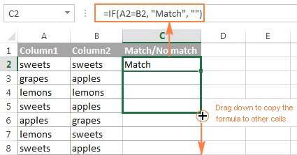
To compare two columns on a row-by-row basis, you’ll start with a simple IF formula comparing the first cells in each column. This formula is then easily applied to the rest of the rows by dragging the fill handle – the small square at the bottom-right corner of the selected cell. When you hover over it, your cursor will change to a plus sign, ready to copy the formula down.
Formula to Highlight Differences
To specifically find rows where the values in two columns are different, use the “not equal to” operator (<>) within the IF function. For instance, to compare cells A2 and B2, the formula would be:
=IF(A2<>B2,"Difference","")
This formula checks if the value in cell A2 is not equal to the value in B2. If they are different, it will display “Difference”; otherwise, it will leave the cell blank.
Formula for Identifying Both Matches and Differences
You can also create a formula that identifies both matches and differences within the same column. This provides a clear overview of your data comparison.
=IF(A2<>B2,"Difference","Match")
Alternatively, you could reverse the logic to prioritize “Match” as the default:
=IF(A2=B2,"Match","Difference")
The results of these formulas will clearly highlight the discrepancies between your columns, as shown below:
Importantly, these formulas work seamlessly with various data types including numbers, dates, times, and text strings.
Tip: For more advanced filtering options when comparing columns row-by-row, explore Excel’s Advanced Filter feature. It offers powerful tools to isolate matches and differences based on complex criteria.
Example 2: Case-Sensitive Difference Checks
The IF formulas we’ve used so far perform case-insensitive comparisons for text values. If you need to differentiate between “Apple” and “apple”, you require a case-sensitive comparison. This is where the EXACT function comes in handy.
To perform a case-sensitive difference check, combine the EXACT function with the IF function.
=IF(EXACT(A2, B2), "", "Case Difference")
In this formula, EXACT(A2, B2) returns TRUE if A2 and B2 are exactly the same (including case), and FALSE otherwise. The IF function then displays “Case Difference” if EXACT returns FALSE (meaning there’s a difference, even if just in case), and leaves the cell blank if they are an exact match.
Comparing Multiple Columns for Differences within Rows
Often, you might need to compare more than two columns within the same row to find differences. Excel provides solutions for various multi-column comparison scenarios.
Example 1: Finding Rows with Any Differences Across Multiple Columns
If you want to identify rows where any of the columns have differing values, the OR function combined with IF is your answer.
For three columns (A, B, and C), the formula would be:
=IF(OR(A2<>B2, B2<>C2, A2<>C2), "Difference in Row", "")
This formula checks all pairwise comparisons between columns A, B, and C. If any of these comparisons result in “TRUE” (meaning a difference), the OR function returns TRUE, and the IF function displays “Difference in Row”.
For a larger number of columns, manually writing out all OR conditions can become cumbersome.
Example 2: Identifying Rows with Differences from the First Column
In scenarios where you want to compare multiple columns against a reference column (e.g., the first column), you can streamline the process. Let’s say column A is your reference, and you want to find rows where columns B, C, D, and E differ from column A.
You can adapt the OR formula or consider a more concise approach if you have many columns. For a large number of columns, consider VBA or Power Query for more efficient solutions, although for a few columns, the OR function is still manageable.
Comparing Two Lists for Differences: Identifying Unique Entries
Let’s shift our focus to comparing two lists in separate columns to find values present in one list but not the other. This is crucial for identifying unique entries or missing data.
For this task, the COUNTIF function is incredibly useful. It allows you to count how many times a value from one column appears in another column.
The core idea is to use COUNTIF to check if a value from column A exists in column B. If the count is zero, it means the value is unique to column A (i.e., it’s a difference when comparing A against B).
=IF(COUNTIF($B:$B, $A2)=0, "Unique to List 1", "")
This formula, placed in a column next to List 1 (column A), checks for each value in column A (starting with A2) whether it exists anywhere in the entire column B ($B:$B). The $ signs ensure that the column B range is absolute, so it doesn’t change when you copy the formula down. If COUNTIF returns 0 (meaning the value from A2 is not found in column B), the IF function displays “Unique to List 1”.
Tip: For larger datasets, specifying a range like $B$2:$B$1000 instead of the entire column $B:$B can improve formula performance.
Alternative formulas for achieving the same result, though potentially less efficient for large datasets, include using ISERROR with MATCH or array formulas with SUM and double negation (--). However, COUNTIF is generally the most straightforward and performant option for this task.
Highlighting Differences Visually with Conditional Formatting
While formulas identify differences textually, Conditional Formatting allows you to visually highlight these discrepancies directly within your Excel sheet. This can make it much easier to quickly spot differences.
Example 1: Highlighting Row Differences
To highlight cells where columns A and B differ in the same row:
- Select the range of cells you want to compare (e.g., columns A and B).
- Go to Home > Conditional Formatting > New Rule.
- Choose “Use a formula to determine which cells to format”.
- Enter the formula:
=$A2<>$B2(assuming row 2 is your first data row). Crucially, use relative row references (no$before the row number) so the formula adjusts for each row. - Click Format to choose your desired highlighting style (e.g., fill color).
- Click OK in both dialog boxes.
This will instantly highlight all cells in your selected range where the values in columns A and B of the same row are different.
To highlight matches instead, simply change the formula to =$A2=$B2.
Example 2: Highlighting Unique Entries in Lists
Conditional Formatting can also highlight unique entries when comparing two lists.
To highlight values in List 1 (column A) that are not in List 2 (column C):
- Select List 1 (column A).
- Create a New Conditional Formatting Rule using the formula:
=COUNTIF($C$2:$C$5, $A2)=0(adjust$C$2:$C$5to the actual range of List 2). - Choose your highlighting format.
Repeat a similar process to highlight unique values in List 2 (column C), using the formula: =COUNTIF($A$2:$A$6, $C2)=0 (adjust $A$2:$A$6 to the actual range of List 1).
Example 3: Highlighting Matches (Duplicates) Between Lists
To highlight values that are present in both lists (duplicates), simply adjust the COUNTIF formulas to look for counts greater than zero.
For List 1 (column A): =COUNTIF($C$2:$C$5, $A2)>0
For List 2 (column C): =COUNTIF($A$2:$A$6, $C2)>0
Highlighting Row Differences and Matches Across Multiple Columns
When dealing with multiple columns, Conditional Formatting remains a powerful tool for visual comparison.
Example 1: Highlighting Rows with Identical Values Across Columns
To highlight entire rows where all columns have the same value:
- Select the data range.
- Create a Conditional Formatting Rule using a formula like:
=COUNTIF($A2:$C2, $A2)=3(for 3 columns A, B, C). Adjust the range and the number3to match your columns. - Set your desired formatting.
Example 2: Quickly Highlighting Row Differences with “Go To Special”
For a lightning-fast way to highlight cells with different values within each row compared to a “comparison column,” Excel’s “Go To Special” feature is invaluable.
- Select your data range.
- Choose your comparison column. By default, the leftmost column in your selection is the comparison column. You can change it by using Tab or Enter to move the active cell (the white cell in the selection) to your desired comparison column.
- Go to Home > Find & Select > Go To Special….
- Select “Row differences” and click OK.
Excel will instantly select all cells that are different from the value in the comparison column within each row. You can then apply a fill color to highlight these differences.
Comparing Two Individual Cells
Comparing two specific cells is a simplified version of row-by-row comparison. You can use the same IF formulas, but without needing to copy them down.
For example, to check if cell A1 is different from cell C1:
=IF(A1<>C1, "Difference", "")
Formula-Free Column Comparison with Specialized Tools
While Excel’s built-in features are powerful, specialized add-ins can further streamline and enhance column comparison tasks, especially for complex scenarios or large datasets. Tools like Ablebits Ultimate Suite offer dedicated features like “Compare Two Tables” that provide a user-friendly interface for advanced comparison options, including highlighting, extracting differences, and merging data.
These tools often go beyond standard Excel functionality, offering more intuitive workflows and features like:
- Multi-column comparison: Compare tables based on multiple key columns.
- Flexible matching options: Configure matching criteria, including fuzzy matching or ignoring case.
- Output options: Highlight differences, extract unique or duplicate values, create summary reports.
These add-ins can significantly boost your efficiency when dealing with frequent or complex column comparison tasks in Excel.
Conclusion
Mastering column comparison in Excel is essential for effective data analysis and data quality management. From simple IF formulas to Conditional Formatting and specialized add-ins, Excel provides a range of tools to suit various comparison needs. By understanding and applying these techniques, you can efficiently identify differences, ensure data accuracy, and gain deeper insights from your spreadsheets. Experiment with these methods to find the most efficient workflows for your specific data comparison challenges in Excel.
Available Downloads
Compare Excel Lists – examples (.xlsx file)
Ultimate Suite – trial version (.exe file)