**What Is The Excel Formula To Compare Two Columns?**

What Is The Excel Formula To Compare Two Columns? Discover effective methods with step-by-step guidance on COMPARE.EDU.VN. Whether identifying duplicates, finding unique entries, or performing row-by-row analysis, leverage Excel’s capabilities to streamline your workflow. Master comparison techniques, enhance data analysis, and make informed decisions with ease, using tools like conditional formatting and lookup functions, enhancing spreadsheet efficiency and data insights, offering practical tips for improving data accuracy.

1. Why Compare Two Columns In Excel?

Excel is a powerful tool for data storage, manipulation, and informed decision-making. Data analysts often rely on Excel to gather crucial information that influences marketing and sales strategies. Comparing two columns in Excel is essential to determine data presence and integrity, especially when dealing with large, interconnected spreadsheets. Manual comparison is time-consuming, potentially taking hours or days to locate missing data. With appropriate formulas and tools, Excel can display results such as TRUE/FALSE or MATCH/NOT MATCH, significantly speeding up the analysis process. This ensures data accuracy and supports better business decisions, making Excel a core asset for professionals needing to analyze and interpret data.

2. How Can I Compare Two Columns In Excel?

There are several ways to compare two columns in Excel, depending on what you need to find. These methods range from highlighting unique or duplicate values to performing row-by-row comparisons. Here’s a brief overview:

Highlighting unique or duplicate values using built-in functions.
Displaying unique or duplicate values using conditional formatting or formulas.
Row-by-row comparison using simple formulas.
Using LOOKUP formulas like VLOOKUP or INDEX-MATCH.

Each method offers a unique way to analyze and compare data, helping you to choose the best approach based on your specific needs.

3. Comparing Two Columns In Excel With Equals Operator

To compare two columns row by row and find matching data, you can use the equals operator (=). This method returns “TRUE” if the values in the compared rows are the same, and “FALSE” if they are different. Here’s how to do it:

Enter the Formula: In the first cell of an empty column (e.g., C2), enter the formula =A2=B2 where A2 and B2 are the first cells in the two columns you want to compare.
Press Enter: Excel will display TRUE or FALSE based on whether the values in A2 and B2 match.
Drag Down the Formula: Click and drag the bottom-right corner of cell C2 down to apply the formula to the rest of the rows.

This method provides a quick and straightforward way to identify matching data across two columns in Excel.

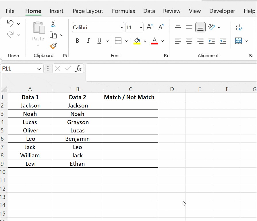
4. How To Compare Two Columns In Excel Using IF Condition

The IF condition is a versatile tool in Excel for comparing two columns and returning specific results based on whether the values match. This method allows you to display custom messages like “Match” or “Not a Match”.

4.1. Identifying Matching Values

To identify matching values, use the formula: =IF(A2=B2,"Match",""). This formula checks if the values in cells A2 and B2 are identical. If they are, the formula returns “Match”; otherwise, it leaves the cell empty.

Enter the Formula: In cell C2, type the formula =IF(A2=B2,"Match","").
Press Enter: If the values in A2 and B2 match, C2 will display “Match”. If they don’t, C2 will remain blank.
Apply to Other Rows: Drag the bottom-right corner of cell C2 down to apply the formula to all corresponding rows.

4.2. Identifying Mismatching Values

To identify mismatching values, you can modify the formula to display a message when the values in the two columns are different. Use the formula: =IF(A2=B2,"Match","Not a Match").

Enter the Formula: In cell C2, enter the formula =IF(A2=B2,"Match","Not a Match").
Press Enter: If A2 and B2 match, C2 will show “Match”. If they don’t, C2 will display “Not a Match”.
Apply to Other Rows: Drag the fill handle (bottom-right corner of C2) down to apply the formula to the rest of the rows.

4.3. Highlighting Differences

You can also use the IF condition to highlight differences between two columns. Replace the equals sign (=) with the non-equality sign (<>) in the IF formula. The formula becomes: =IF(A2<>B2,"Not a Match","Match").

Enter the Formula: In cell C2, type the formula =IF(A2<>B2,"Not a Match","Match").
Press Enter: If A2 and B2 are different, C2 will display “Not a Match”. If they are the same, C2 will display “Match”.
Apply to Other Rows: Drag the fill handle from C2 down to apply the formula to all rows.

These formulas provide a clear way to compare data and identify matches and mismatches, making data analysis more efficient.

5. Compare Two Columns In Excel Using EXACT() Function

When comparing two columns in Excel, the EXACT() function is crucial for case-sensitive comparisons. Standard formulas like A2=B2 are case-insensitive, meaning they treat “Text” and “text” as the same. The EXACT() function, however, differentiates between uppercase and lowercase letters.

5.1. How the EXACT() Function Works

The EXACT() function compares two text strings and returns TRUE if they are identical, including case, and FALSE otherwise. The syntax is =EXACT(text1, text2), where text1 and text2 are the strings you want to compare.

Text1: The first text string.
Text2: The second text string.

5.2. Using EXACT() with an IF Condition

To make the comparison more informative, you can use EXACT() with an IF condition to return custom messages like “Match” or “Mismatch”. The formula structure is =IF(EXACT(A2, B2), "Match", "Mismatch").

Enter the Formula: In cell C2, enter the formula =IF(EXACT(A2, B2), "Match", "Mismatch").
Press Enter: Excel will display “Match” if the text in A2 and B2 are exactly the same (including case) and “Mismatch” if they are different.
Apply to Other Rows: Drag the fill handle (the bottom-right corner of cell C2) down to apply the formula to the rest of the rows.

5.3. Example Scenario

Consider two columns, Data1 and Data2, containing similar text strings.

	Column A (Data1)	Column B (Data2)	Column C (Result)
Row 2	Nova Scotia	Nova Scotia	Match (Case-Insensitive)
Row 2	Nova Scotia	nova scotia	Mismatch (Case-Sensitive)

Case-Insensitive Comparison: The formula =IF(A2=B2, "Match", "Mismatch") returns “Match” because it ignores case differences.
Case-Sensitive Comparison: The formula =IF(EXACT(A2, B2), "Match", "Mismatch") returns “Mismatch” because it considers the case difference between “Nova Scotia” and “nova scotia”.

5.4. How the Formula Executes

The IF condition first executes the inner function, EXACT(), which returns TRUE or FALSE. Based on this result, the IF condition returns the corresponding message. If EXACT() returns TRUE, the IF condition returns “Match”; otherwise, it returns “Mismatch”.

6. Compare Two Columns In Excel Using Conditional Formatting

Conditional formatting is a powerful Excel feature that allows you to highlight cells based on specific criteria. This is particularly useful when comparing two columns for duplicate or unique values without needing a third column for results.

6.1. Highlighting Duplicate Values

To highlight values that appear in both columns, follow these steps:

Select the Columns: Select both columns of data that you want to compare.
Open Conditional Formatting: Go to Home > Styles > Conditional Formatting > Highlight Cells Rules > Duplicate Values.
Choose Formatting: In the dialog box, ensure “Duplicate” is selected in the first dropdown menu. Choose a formatting style (e.g., light red fill with dark red text) from the second dropdown menu or select “Custom Format” to create a custom style.
Apply Formatting: Click OK to apply the formatting.

Excel will now highlight all values that appear in both columns, making it easy to spot common entries.

6.2. Highlighting Unique Values

To highlight values that appear only in one of the columns (unique values), follow these steps:

Select the Columns: Select both columns of data.
Open Conditional Formatting: Go to Home > Styles > Conditional Formatting > Highlight Cells Rules > Duplicate Values.
Choose “Unique”: In the dialog box, select “Unique” from the first dropdown menu.
Choose Formatting: Choose a formatting style or create a custom format.
Apply Formatting: Click OK to apply the formatting.

Excel will now highlight all values that are unique to each column, allowing you to quickly identify distinct entries.

6.3. Clearing Conditional Formatting

To remove conditional formatting from the cells, follow these steps:

Select the Cells: Select the cells from which you want to remove the formatting.
Clear Rules: Go to Conditional Formatting > Clear Rules > Clear Rules from Selected Cells.

This will remove any conditional formatting rules applied to the selected cells.

6.4. Benefits of Using Conditional Formatting

Visual Identification: Quickly see matching or unique data without needing extra columns.
Dynamic Updates: Formatting automatically updates as data changes.
Ease of Use: Simple to set up and clear formatting rules.

7. Using Lookup Function To Compare Two Columns

Lookup functions in Excel are essential for comparing data across columns by searching for specific values and returning corresponding information. Functions like VLOOKUP, HLOOKUP, and XLOOKUP are particularly useful.

7.1. Understanding Lookup Functions

VLOOKUP (Vertical Lookup): Searches for a value in the first column of a range and returns a value from any cell on the same row of that range.
HLOOKUP (Horizontal Lookup): Searches for a value in the top row of a range and returns a value from any cell in the same column of that range.
XLOOKUP: A more versatile function that combines the capabilities of both VLOOKUP and HLOOKUP, offering improved flexibility and ease of use.

7.2. Using VLOOKUP to Compare Columns

Consider two columns: Column A contains a list of exams taken by a student, and Column B contains a list of subjects the student passed. You can use VLOOKUP to determine which exams the student has cleared.

Formula: Enter the following formula in cell C2: =VLOOKUP(A2, $B$2:$B$5, 1, 0)
- A2: The lookup value (the exam name in Column A).
- $B$2:$B$5: The table array (the range of cells containing the list of passed subjects in Column B). The $ signs create an absolute reference, ensuring the range doesn’t change when you drag the formula.
- 1: The column index number (the column from which to return a value). In this case, it’s 1 because we’re looking up values in a single column.
- 0: The range lookup value (0 for an exact match, 1 for an approximate match).
Apply to Other Rows: Drag the formula down from C2 to apply it to all the rows in Column C.

If the exam in Column A is found in Column B (meaning the student passed the subject), VLOOKUP will return the subject name. If the exam is not found, VLOOKUP will return #N/A.

7.3. Interpreting the Results

If cell C2 displays a subject name, it means the student passed that subject.
If cell C2 displays #N/A, it means the student has not passed that subject.

7.4. Key Components of the VLOOKUP Formula

VLOOKUP(lookup_value, table_array, col_index_num, [range_lookup])
- lookup_value: The value you want to find.
- table_array: The range of cells where you want to look for the value.
- col_index_num: The column number in the table array from which to return a value.
- range_lookup: A logical value that specifies whether you want to find an exact match (FALSE or 0) or an approximate match (TRUE or 1).

7.5. Absolute References

The $ symbol is used to create absolute references. When you use absolute references, the cell references in the formula do not change when you copy or drag the formula to other cells. This is important when you want to keep the table array constant.

8. What Are Some Other Methods To Compare Two Columns In Excel Using The IF Condition?

To find matches in all cells within the same row when the table has three or more columns when you want to find rows with the same values in all cells, use an IF formula with an AND statement. The formula is =IF(AND(A2=B2, A2=C2), “Full match”, “”).

And the formula to find matches in any two cells in the same row is =IF(OR(A2=B2, B2=C2, A2=C2), “Match”, “”).

8.1. Using IF with AND for Full Match

The AND function checks whether all conditions within it are true. When combined with the IF function, you can verify if all specified columns in a row have matching values.

Enter the Formula: In cell D2, enter the formula =IF(AND(A2=B2, A2=C2), "Full Match", "").
Press Enter: The formula will display “Full Match” if the values in cells A2, B2, and C2 are identical. If any of the values differ, the cell will remain blank.
Apply to Other Rows: Drag the fill handle down from D2 to apply the formula to the rest of the rows.

8.2. Using IF with OR for Any Match

The OR function checks whether at least one of the conditions within it is true. This is useful for identifying rows where any two columns have matching values.

Enter the Formula: In cell D2, enter the formula =IF(OR(A2=B2, B2=C2, A2=C2), "Match", "").
Press Enter: The formula will display “Match” if any two of the cells A2, B2, or C2 have the same value. If none of the cells match, the cell will remain blank.
Apply to Other Rows: Drag the fill handle down from D2 to apply the formula to the rest of the rows.

9. Compare Two Columns In Excel Using The Index-Match Function?

The INDEX-MATCH function is a powerful alternative to VLOOKUP for comparing two columns in different tables and pulling matching entries. Unlike VLOOKUP, INDEX-MATCH is more flexible and avoids the limitations of having to search in the first column of the table array.

9.1. How INDEX-MATCH Works

MATCH: This function searches for a specified item in a range of cells and returns the relative position of that item in the range.
INDEX: This function returns the value of a cell in a table based on the row and column number you specify.

9.2. Formula Structure

The general structure of the INDEX-MATCH formula for comparing two columns is:

=INDEX(return_column, MATCH(lookup_value, lookup_column, 0))

return_column: The range of cells from which to return a value.
lookup_value: The value you want to find.
lookup_column: The range of cells where you want to look for the value.
0: Specifies that you want an exact match.

9.3. Example Scenario

Suppose you have two tables: Table 1 contains a list of IDs in Column A and corresponding names in Column B, and Table 2 contains a list of IDs in Column D. You want to find the names from Table 1 that match the IDs in Table 2.

Enter the Formula: In cell E2 (in Table 2), enter the following formula: =INDEX($B$2:$B$4, MATCH(D2, $A$2:$A$4, 0))
- $B$2:$B$4: The range of cells containing the names you want to return (Column B in Table 1).
- D2: The lookup value (the ID in Column D of Table 2).
- $A$2:$A$4: The range of cells where you want to look for the ID (Column A in Table 1).
- 0: Specifies that you want an exact match.
Apply to Other Rows: Drag the formula down from E2 to apply it to all the rows in Column E.

9.4. Interpreting the Results

If the ID in Column D of Table 2 is found in Column A of Table 1, the corresponding name from Column B will be displayed in Column E.
If the ID is not found, the formula will return #N/A.

9.5. Advantages of INDEX-MATCH over VLOOKUP

Flexibility: INDEX-MATCH can look up values to the left, whereas VLOOKUP can only look to the right.
Efficiency: INDEX-MATCH only looks at the necessary columns, making it faster, especially for large datasets.
Robustness: INDEX-MATCH is less likely to break if columns are inserted or deleted in the table.

By using INDEX-MATCH, you can efficiently compare data across different tables and retrieve corresponding values, enhancing your data analysis capabilities in Excel.

FAQ: Comparing Columns in Excel

1. How can I quickly compare two columns in Excel to find differences?

To quickly compare two columns in Excel and highlight the differences, select both columns, then go to Home → Find & Select → Go To Special → Row Differences, and click OK. The matching cells will remain white, while the unmatched cells will be highlighted in gray.

2. Can I compare two columns in Excel using a formula that returns “Match” or “No Match”?

Yes, you can use the IF function to compare two columns and return “Match” or “No Match”. The formula is =IF(A2=B2, "Match", "No Match"). This formula compares the values in cells A2 and B2. If they are the same, it returns “Match”; otherwise, it returns “No Match”.

3. How do I compare two columns in Excel for case-sensitive matches?

To perform a case-sensitive comparison, use the EXACT function within an IF statement. The formula is =IF(EXACT(A2, B2), "Match", "No Match"). The EXACT function checks if two text strings are identical, including case.

4. Is it possible to highlight duplicate values in two columns using conditional formatting?

Yes, you can highlight duplicate values in two columns using conditional formatting. Select both columns, then go to Home → Conditional Formatting → Highlight Cells Rules → Duplicate Values. Choose the formatting style you prefer, and click OK.

5. How can I compare two columns in Excel and return a value from another column if there is a match?

You can use the VLOOKUP function for this purpose. For example, if you want to compare column A with column B and return a value from column C when there is a match, the formula would be =VLOOKUP(A2, B:C, 2, FALSE).

6. What is the difference between VLOOKUP and INDEX-MATCH for comparing columns?

VLOOKUP searches for a value in the first column of a range and returns a value from another column in the same row. INDEX-MATCH is more flexible because it can look up values in any column and return a value from any other column, making it more robust and efficient.

7. How can I use conditional formatting to highlight unique values in two columns?

Select both columns, then go to Home → Conditional Formatting → Highlight Cells Rules → Duplicate Values. In the dialog box, select “Unique” instead of “Duplicate”. Choose the formatting style, and click OK.

8. Can I compare two columns in Excel to find values that are present in one column but not in the other?

Yes, you can use a combination of COUNTIF and IF functions to achieve this. For example, to find values in column A that are not in column B, use the formula =IF(COUNTIF(B:B, A2)=0, "Not Found", ""). This formula checks if the value in A2 exists in column B. If it doesn’t, it returns “Not Found”.

9. How do I compare two columns in different Excel sheets?

You can use the same formulas as comparing columns in the same sheet, but you need to specify the sheet name in the formula. For example, to compare column A in Sheet1 with column A in Sheet2, the formula would be =IF(Sheet1!A2=Sheet2!A2, "Match", "No Match").

10. Is there a way to compare two columns and ignore differences in spaces or special characters?

You can use the TRIM and SUBSTITUTE functions to remove spaces and special characters before comparing the columns. For example, the formula =IF(TRIM(A2)=TRIM(B2), "Match", "No Match") removes leading and trailing spaces before comparing the values.

Conclusion

Comparing two columns in Excel is a common and essential task for data analysis, and Excel offers a variety of methods to accomplish this efficiently. From simple formulas like A2=B2 and IF conditions to more advanced functions like EXACT, VLOOKUP, and INDEX-MATCH, each technique provides unique advantages for different scenarios. Conditional formatting offers a visual approach to highlight duplicate or unique values, while lookup functions allow you to compare data across different tables and retrieve corresponding information. By mastering these methods, you can streamline your data analysis workflow, ensure data accuracy, and make informed decisions.

For those looking to deepen their Excel skills and explore more advanced techniques, COMPARE.EDU.VN offers comprehensive guides and resources. Whether you’re a beginner or an experienced user, our platform provides the knowledge and tools you need to enhance your spreadsheet proficiency and gain deeper insights from your data.

Ready to take your Excel skills to the next level? Visit COMPARE.EDU.VN today to discover more tutorials, tips, and courses. Make informed decisions with confidence using the power of Excel. Contact us at 333 Comparison Plaza, Choice City, CA 90210, United States. Reach out via WhatsApp at +1 (626) 555-9090 or explore our website at compare.edu.vn for more information.