How Can Vlookup Be Used To Compare Two Columns?

Vlookup can be used to compare two columns to find matches and differences efficiently. At COMPARE.EDU.VN, we provide comprehensive guides to help you master Vlookup and other powerful Excel functions. This allows you to quickly identify common entries, locate missing data, and streamline your data analysis. Learn how to leverage Vlookup for precise data comparisons and enhanced productivity. Understand related techniques like index match, data comparison and error handling.

1. Understanding the Basics of VLOOKUP for Column Comparison

VLOOKUP is a versatile Excel function used to search for a value in the first column of a range and return a value from a specified column in the same row. When comparing two columns, VLOOKUP can help identify common values or find data missing in one of the columns. Its primary function is to look up data, making it ideal for matching entries between different datasets.

1.1. What is VLOOKUP and How Does It Work?

VLOOKUP stands for “Vertical Lookup.” It works by searching for a specific value in the leftmost column of a table and then returning a value in the same row from a column you specify. The syntax of the VLOOKUP function is as follows:

=VLOOKUP(lookup_value, table_array, col_index_num, [range_lookup])

lookup_value: The value you want to search for.
table_array: The range of cells where you want to search.
col_index_num: The column number in the range from which to return a value.
range_lookup: A logical value (TRUE or FALSE) that specifies whether you want an approximate or exact match. FALSE for exact match is highly recommended when comparing columns for accurate results.

1.2. Key Components of the VLOOKUP Formula

To effectively use VLOOKUP for column comparison, it’s essential to understand each component:

Lookup Value: This is the value you are trying to find in another column.
Table Array: This is the range containing the column you are searching in and the column from which you want to return a value. Always use absolute references (e.g., $A$1:$B$10) to prevent the range from changing when you copy the formula.
Column Index Number: This specifies which column in the table array contains the value you want to return. For example, if your table array is two columns wide, and you want to return the value from the second column, you would enter 2.
Range Lookup: Set this to FALSE for an exact match. This ensures that VLOOKUP only returns a value if it finds an exact match for the lookup value.

1.3. Preparing Your Data for VLOOKUP

Before using VLOOKUP, ensure your data is properly prepared:

Ensure the Lookup Value is in the First Column: VLOOKUP only searches in the first column of the table array.
Remove Duplicates: Remove any duplicate entries from the column you are searching in to avoid incorrect matches.
Sort Data (If Necessary): If you are using an approximate match (range_lookup set to TRUE), the first column of the table array must be sorted in ascending order.
Consistent Data Types: Ensure that the data types in both columns being compared are consistent. For example, if one column contains numbers formatted as text, convert them to numbers.

2. Step-by-Step Guide: Using VLOOKUP to Compare Two Columns

Here’s a detailed guide on how to use Vlookup To Compare Two Columns in Excel, with practical examples.

2.1. Scenario: Identifying Common Values

Suppose you have two lists of customer IDs in columns A and B, and you want to find out which IDs are present in both lists.

Set Up Your Data:
- Column A: List 1 (e.g., customer IDs)
- Column B: List 2 (e.g., customer IDs)
Enter the VLOOKUP Formula:
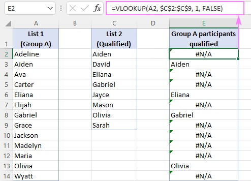
- In cell C2, enter the following formula:
  =VLOOKUP(A2, $B$2:$B$10, 1, FALSE)
- Here, A2 is the lookup value (the first customer ID in List 1), $B$2:$B$10 is the table array (List 2), 1 is the column index number (since we’re looking for the ID itself), and FALSE specifies an exact match.
Drag the Formula Down:
- Drag the formula from C2 down to apply it to all the customer IDs in List 1.
Interpret the Results:
- If VLOOKUP finds a match, it returns the customer ID from List 2.
- If VLOOKUP does not find a match, it returns a #N/A error.

2.2. Scenario: Finding Missing Values

Now, let’s find out which customer IDs from List 1 are not present in List 2.

Set Up Your Data:
- Column A: List 1 (e.g., customer IDs)
- Column B: List 2 (e.g., customer IDs)
Enter the VLOOKUP Formula with ISNA:
- In cell C2, enter the following formula:
  =IF(ISNA(VLOOKUP(A2, $B$2:$B$10, 1, FALSE)), "Not Found", "Found")
- This formula uses the ISNA function to check for #N/A errors. If VLOOKUP returns an error (meaning the customer ID is not found in List 2), ISNA returns TRUE, and the IF function displays “Not Found”. Otherwise, it displays “Found”.
Drag the Formula Down:
- Drag the formula from C2 down to apply it to all the customer IDs in List 1.
Interpret the Results:
- “Not Found” indicates that the customer ID is present in List 1 but not in List 2.
- “Found” indicates that the customer ID is present in both List 1 and List 2.

2.3. Dealing with #N/A Errors

The #N/A error can be unsightly and confusing. Here are a couple of ways to handle it:

Using IFNA (Excel 2013 and later):
- The IFNA function allows you to specify a value to return if VLOOKUP results in an #N/A error.
- Example:
  =IFNA(VLOOKUP(A2, $B$2:$B$10, 1, FALSE), "Not Found")
Using IFERROR (Excel 2007 and later):
- The IFERROR function is similar to IFNA but can handle all types of errors, not just #N/A.
- Example:
  =IFERROR(VLOOKUP(A2, $B$2:$B$10, 1, FALSE), "Not Found")

2.4. Comparing Columns in Different Excel Sheets

Sometimes, the columns you need to compare are located in different sheets. Here’s how to handle that:

Set Up Your Data:
- Sheet1: List 1 (e.g., customer IDs in column A)
- Sheet2: List 2 (e.g., customer IDs in column A)
Enter the VLOOKUP Formula:
- In Sheet1, cell B2, enter the following formula:
  =IFNA(VLOOKUP(A2, Sheet2!$A$2:$A$10, 1, FALSE), "Not Found")
- This formula references the range in Sheet2 using the syntax Sheet2!$A$2:$A$10.
Drag the Formula Down:
- Drag the formula from B2 down to apply it to all the customer IDs in List 1.
Interpret the Results:
- “Not Found” indicates that the customer ID is present in Sheet1 but not in Sheet2.
- The customer ID indicates that the customer ID is present in both Sheet1 and Sheet2.

3. Advanced VLOOKUP Techniques for Data Comparison

To further enhance your data comparison skills, explore these advanced techniques.

3.1. Using VLOOKUP with Multiple Criteria

VLOOKUP can only look up values based on one criterion. To compare columns based on multiple criteria, you can create a helper column that concatenates the criteria into a single value.

Set Up Your Data:
- Column A: List 1 – Criterion 1
- Column B: List 1 – Criterion 2
- Column D: List 2 – Criterion 1
- Column E: List 2 – Criterion 2
Create a Helper Column in Both Lists:
- In column C (List 1), enter the formula:
  =A2&"|"&B2
- In column F (List 2), enter the formula:
  =D2&"|"&E2
- The &"|" concatenates the two criteria with a separator (“|”) to ensure uniqueness.
Use VLOOKUP on the Helper Columns:
- In cell G2, enter the following formula:
  =IFNA(VLOOKUP(C2, $F$2:$F$10, 1, FALSE), "Not Found")
- This formula looks up the concatenated value from List 1 in the concatenated values of List 2.
Drag the Formula Down:
- Drag the formula from G2 down to apply it to all the entries in List 1.

3.2. Combining VLOOKUP with Other Functions (e.g., MATCH, INDEX)

While VLOOKUP is useful, it has limitations. Combining it with other functions like MATCH and INDEX can provide more flexibility.

INDEX and MATCH:
- The INDEX and MATCH functions can perform lookups more flexibly than VLOOKUP. MATCH finds the position of a value in a range, and INDEX returns the value at a specific position in a range.
- Example:
  =IFNA(INDEX($E$2:$E$10, MATCH(A2, $D$2:$D$10, 0)), "Not Found")
- Here, MATCH finds the row number where A2 is found in $D$2:$D$10, and INDEX returns the corresponding value from $E$2:$E$10.
XLOOKUP (Excel 365 and later):
- XLOOKUP is a modern function that combines the capabilities of VLOOKUP and INDEX/MATCH, providing more flexibility and ease of use.
- Example:
  =XLOOKUP(A2, $D$2:$D$10, $E$2:$E$10, "Not Found")
- This formula looks up A2 in $D$2:$D$10 and returns the corresponding value from $E$2:$E$10, or “Not Found” if no match is found.

3.3. Using Dynamic Arrays with VLOOKUP (Excel 365)

Excel 365 introduces dynamic arrays, which can simplify complex formulas. Here’s how to use them with VLOOKUP:

Finding Common Values with FILTER:
- =FILTER(A2:A10, NOT(ISNA(VLOOKUP(A2:A10, B2:B10, 1, FALSE))))
- This formula returns an array of values from A2:A10 that are found in B2:B10.
Finding Missing Values with FILTER:
- =FILTER(A2:A10, ISNA(VLOOKUP(A2:A10, B2:B10, 1, FALSE)))
- This formula returns an array of values from A2:A10 that are not found in B2:B10.

4. Best Practices for Efficient Column Comparison with VLOOKUP

Follow these best practices to ensure your column comparisons are accurate and efficient.

4.1. Ensuring Data Integrity

Data Validation: Use data validation to restrict the type of data entered in your columns, reducing errors and inconsistencies.
Data Cleaning: Regularly clean your data to remove duplicates, correct errors, and standardize formats.
Consistent Formatting: Ensure that the data being compared has consistent formatting.

4.2. Optimizing VLOOKUP Performance

Use Exact Match (FALSE): Always use FALSE for range_lookup unless you specifically need an approximate match.
Sort Data (If Using Approximate Match): If you use TRUE for range_lookup, ensure the lookup column is sorted in ascending order.
Limit Table Array Size: Keep the table array as small as possible to improve performance.
Use Helper Columns Wisely: While helper columns can be useful, avoid creating too many, as they can slow down your spreadsheet.

4.3. Error Handling and Troubleshooting

Check for #N/A Errors: Use IFNA or IFERROR to handle #N/A errors gracefully.
Verify Lookup Value and Table Array: Double-check that the lookup value and table array are correct.
Ensure Correct Column Index Number: Make sure the column index number is accurate.
Use Evaluate Formula: Use Excel’s Evaluate Formula tool to step through the VLOOKUP calculation and identify any issues.

5. Alternative Methods for Comparing Two Columns

While VLOOKUP is a powerful tool, several alternative methods can be used to compare two columns in Excel.

5.1. Using Conditional Formatting

Conditional formatting can highlight differences or common values directly in your columns.

Highlight Common Values:
- Select the first column.
- Go to Home > Conditional Formatting > Highlight Cells Rules > Duplicate Values.
- Choose a formatting style to highlight common values.
- Repeat for the second column.
Highlight Unique Values:
- Select the first column.
- Go to Home > Conditional Formatting > Highlight Cells Rules > Duplicate Values.
- Change “Duplicate” to “Unique.”
- Choose a formatting style to highlight unique values.
- Repeat for the second column.

5.2. Using COUNTIF Function

The COUNTIF function counts the number of cells within a range that meet a given criterion.

Set Up Your Data:
- Column A: List 1
- Column B: List 2
Enter the COUNTIF Formula:
- In cell C2, enter the following formula:
  =COUNTIF($B$2:$B$10, A2)
- This formula counts how many times A2 appears in the range $B$2:$B$10.
Drag the Formula Down:
- Drag the formula from C2 down to apply it to all the entries in List 1.
Interpret the Results:
- If the result is greater than 0, the value is present in both lists.
- If the result is 0, the value is not present in List 2.

5.3. Using the MATCH Function

The MATCH function returns the position of a specified value in a range.

Set Up Your Data:
- Column A: List 1
- Column B: List 2
Enter the MATCH Formula:
- In cell C2, enter the following formula:
  =IFNA(MATCH(A2, $B$2:$B$10, 0), "Not Found")
- This formula finds the position of A2 in the range $B$2:$B$10. If A2 is not found, it returns “Not Found”.
Drag the Formula Down:
- Drag the formula from C2 down to apply it to all the entries in List 1.

6. Real-World Applications of VLOOKUP for Column Comparison

VLOOKUP’s column comparison capabilities are valuable in various industries and scenarios.

6.1. Financial Analysis

Reconciling Transactions: Compare transaction lists from different sources to identify discrepancies.
Auditing Data: Verify the accuracy of financial data by comparing it against other datasets.
Analyzing Sales Data: Compare sales data across different periods to identify trends and anomalies.

6.2. Inventory Management

Tracking Inventory Levels: Compare inventory lists to identify missing items or discrepancies.
Managing Stock Levels: Compare current stock levels against reorder points to ensure adequate supply.
Identifying Discrepancies: Resolve differences between physical stock counts and recorded inventory levels.

6.3. Human Resources

Comparing Employee Lists: Identify employees who are present in one list but not another.
Tracking Training Records: Compare training records against employee lists to ensure compliance.
Analyzing Performance Data: Compare performance metrics across different teams or departments.

6.4. Sales and Marketing

Lead Management: Compare lead lists from different sources to identify duplicates.
Customer Data Analysis: Compare customer data across different systems to create a unified view.
Campaign Performance: Compare campaign results against target metrics to assess effectiveness.

7. Common Mistakes to Avoid When Using VLOOKUP

To ensure accurate and efficient column comparisons, avoid these common mistakes when using VLOOKUP.

7.1. Incorrect Range Lookup Value

Mistake: Using TRUE for range_lookup when you need an exact match.
Solution: Always use FALSE for exact matches. Only use TRUE if you specifically need an approximate match and the lookup column is sorted.

7.2. Using Relative References Instead of Absolute References

Mistake: Using relative references in the table_array, causing the range to shift when the formula is dragged down.
Solution: Always use absolute references (e.g., $A$1:$B$10) for the table_array.

7.3. Forgetting to Lock the Table Array

Mistake: Failing to lock the table array when dragging the formula, leading to incorrect results.
Solution: Use the $ symbol to lock the column and row references (e.g., $A$1:$B$10).

7.4. Inconsistent Data Types

Mistake: Comparing data with inconsistent data types (e.g., numbers formatted as text).
Solution: Ensure that the data types in both columns being compared are consistent. Use the VALUE function or format cells as numbers.

7.5. Errors in the Lookup Column

Mistake: Presence of errors in the lookup column, causing VLOOKUP to return incorrect results.
Solution: Clean and validate your data to remove duplicates, correct errors, and standardize formats.

7.6. Not Handling Errors

Mistake: Not using IFNA or IFERROR to handle #N/A errors, resulting in a messy and confusing spreadsheet.
Solution: Use IFNA or IFERROR to display a more user-friendly message when no match is found.

8. Optimizing Your Workflow with COMPARE.EDU.VN

At COMPARE.EDU.VN, we understand the importance of efficient data comparison. That’s why we offer a range of resources to help you master VLOOKUP and other Excel functions.

8.1. Why Choose COMPARE.EDU.VN?

Comprehensive Guides: Our detailed guides provide step-by-step instructions for using VLOOKUP and other Excel functions.
Practical Examples: We offer practical examples that demonstrate how to apply VLOOKUP in real-world scenarios.
Advanced Techniques: Learn advanced techniques to enhance your data comparison skills.
Best Practices: Follow our best practices to ensure accurate and efficient column comparisons.
Real-World Applications: Discover how VLOOKUP can be used in various industries and scenarios.

8.2. How COMPARE.EDU.VN Can Help You Master VLOOKUP

Detailed Tutorials: Access our detailed tutorials on VLOOKUP and other Excel functions.
Step-by-Step Instructions: Follow our step-by-step instructions to perform column comparisons with VLOOKUP.
Advanced Tips and Tricks: Learn advanced tips and tricks to optimize your VLOOKUP performance.
Error Handling Techniques: Discover how to handle errors and troubleshoot common issues.

9. Frequently Asked Questions (FAQs) About VLOOKUP for Column Comparison

9.1. Can VLOOKUP Compare Two Columns?

Yes, VLOOKUP can compare two columns to find common values or identify missing data in one of the columns. By using VLOOKUP, you can quickly determine which values from one column exist in another.

9.2. How Do I Use VLOOKUP to Find Missing Values?

To use VLOOKUP to find missing values, nest the VLOOKUP formula within an IF and ISNA function. This will return a specific value (e.g., “Not Found”) if VLOOKUP results in an #N/A error, indicating that the value is missing.

9.3. How Do I Handle #N/A Errors in VLOOKUP?

You can handle #N/A errors in VLOOKUP using the IFNA (Excel 2013 and later) or IFERROR (Excel 2007 and later) functions. These functions allow you to specify a value to return if VLOOKUP results in an error.

9.4. Can I Compare Columns in Different Excel Sheets Using VLOOKUP?

Yes, you can compare columns in different Excel sheets using VLOOKUP. Simply reference the range in the other sheet using the syntax SheetName!Range.

9.5. How Can I Compare Two Columns Based on Multiple Criteria?

To compare two columns based on multiple criteria, create a helper column in both lists that concatenates the criteria into a single value. Then, use VLOOKUP to compare the helper columns.

9.6. What Are Some Alternatives to VLOOKUP for Column Comparison?

Alternatives to VLOOKUP for column comparison include conditional formatting, COUNTIF, MATCH, and dynamic arrays with FILTER.

9.7. How Do I Optimize VLOOKUP Performance?

To optimize VLOOKUP performance, use exact match (FALSE), sort data if using approximate match, limit table array size, and use helper columns wisely.

9.8. How Do I Ensure Data Integrity When Using VLOOKUP?

To ensure data integrity, use data validation, clean your data regularly, and ensure consistent formatting.

9.9. What Are Common Mistakes to Avoid When Using VLOOKUP?

Common mistakes to avoid when using VLOOKUP include incorrect range lookup value, using relative references instead of absolute references, forgetting to lock the table array, inconsistent data types, errors in the lookup column, and not handling errors.

9.10. Can I Use VLOOKUP with Dynamic Arrays in Excel 365?

Yes, you can use VLOOKUP with dynamic arrays in Excel 365 to simplify complex formulas and perform more flexible column comparisons.

10. Conclusion: Mastering Column Comparison with VLOOKUP

Mastering VLOOKUP for column comparison can significantly enhance your data analysis skills in Excel. By understanding the basics, following best practices, and exploring advanced techniques, you can efficiently identify common values, find missing data, and streamline your workflow.

At COMPARE.EDU.VN, we are committed to providing you with the resources you need to excel in data comparison. Explore our comprehensive guides, practical examples, and advanced tips to unlock the full potential of VLOOKUP and other Excel functions. Start leveraging VLOOKUP today and take your data analysis skills to the next level.

Ready to dive deeper into the world of data comparison? Visit COMPARE.EDU.VN now to explore our detailed tutorials and resources. Whether you’re reconciling financial transactions, managing inventory levels, or analyzing sales data, our guides will help you make informed decisions and achieve your goals. Don’t miss out on the opportunity to enhance your skills and optimize your workflow with COMPARE.EDU.VN.

Address: 333 Comparison Plaza, Choice City, CA 90210, United States

Whatsapp: +1 (626) 555-9090

Website: compare.edu.vn