Using VLOOKUP to compare two Excel sheets is a straightforward method for identifying differences and discrepancies in your data. At compare.edu.vn, we’ll break down the process into easy-to-follow steps, enabling you to reconcile data effectively. By using VLOOKUP, or XLOOKUP, users can ensure the accuracy of their Excel spreadsheets. We provide simple, effective methods that make data analysis easy. Understand data analysis, reconciliation techniques, and comparison methods.
1. What Is VLOOKUP and Why Use It for Comparing Excel Sheets?
VLOOKUP (Vertical Lookup) is an Excel function that searches for a specific value in the first column of a range and returns a value from a cell in the same row, based on a specified column number. It’s highly useful for comparing data across two Excel sheets, allowing you to quickly identify matching or differing entries based on a unique identifier. This function is essential in data analysis.
VLOOKUP is valuable for several reasons:
- Efficiency: Quickly compares large datasets.
- Accuracy: Reduces manual errors.
- Identification of Discrepancies: Highlights differences between sheets.
- Data Reconciliation: Simplifies the process of aligning data.
2. Defining Your Comparison Goals in Excel
Before diving into the technical steps, it’s important to clearly define what you aim to achieve with your comparison. Understanding your goals ensures that you use VLOOKUP effectively and interpret the results accurately.
2.1. Identify Key Data Fields
Determine which columns in your Excel sheets contain the data you want to compare. Common fields include:
- Customer IDs: Unique identifiers for customers.
- Invoice Numbers: Unique identifiers for invoices.
- Product Codes: Unique identifiers for products.
- Dates: Transaction dates, delivery dates, etc.
- Amounts: Financial values, quantities, etc.
2.2. Determine the Type of Comparison
Decide whether you need to:
- Verify Matches: Ensure the same data exists in both sheets.
- Identify Differences: Find discrepancies in corresponding fields.
- Locate Missing Entries: Determine records present in one sheet but not the other.
- Reconcile Values: Align data between the two sheets based on certain criteria.
2.3. Define Your Expected Outcome
Clearly define the expected outcome of your comparison. For instance, you might want to:
- Generate a list of matching records.
- Produce a report of discrepancies.
- Update one sheet with missing data from the other.
- Identify errors in data entry.
Having a clear understanding of your goals will guide you in setting up your VLOOKUP formulas and interpreting the results effectively.
3. Preparing Your Excel Sheets for Comparison
To effectively use VLOOKUP, your Excel sheets need to be properly structured. Preparation ensures accurate comparisons and simplifies the reconciliation process.
3.1. Organize Your Data
Ensure both Excel sheets have a similar layout with consistent column headers. This standardization is crucial for VLOOKUP to work accurately.
- Consistent Headers: Column headers should be identical across both sheets. For example, if one sheet uses “Customer ID,” the other should not use “Cust ID.”
- Data Types: Ensure data types are consistent. For example, if “Amount” is formatted as currency in one sheet, it should be the same in the other.
- Clean Data: Remove any unnecessary rows or columns that are not relevant to the comparison.
3.2. Identify a Unique Identifier Column
A unique identifier is a column that contains distinct values for each row, such as Customer ID, Invoice Number, or Product Code. This column is critical for VLOOKUP to locate matching records between the two sheets.
- Ensure Uniqueness: Verify that the identifier column contains no duplicates. Duplicates can lead to inaccurate VLOOKUP results.
- Consistency: The unique identifier should be present and consistently formatted in both sheets.
3.3. Sort Your Data (Optional)
Sorting your data by the unique identifier column can sometimes improve VLOOKUP’s performance, especially with large datasets. While not always necessary, it can make the comparison process more efficient.
- Ascending Order: Sort both sheets in ascending order by the unique identifier.
- Consistent Sorting: Ensure both sheets are sorted in the same way to maintain alignment.
3.4. Create a New Worksheet for Comparison
It’s good practice to perform the comparison in a new worksheet to avoid altering the original data. This also helps in keeping the results organized and easy to review.
- New Tab: Insert a new worksheet in your Excel workbook.
- Copy Headers: Copy the headers from one of your data sheets to the new worksheet.
By following these preparation steps, you ensure that your data is well-organized and ready for the VLOOKUP comparison, leading to more accurate and reliable results.
4. Step-by-Step Guide: Using VLOOKUP to Compare Data
This section provides a detailed, step-by-step guide on how to use VLOOKUP to compare data between two Excel sheets. Follow these instructions carefully to achieve accurate and efficient comparisons.
4.1. Setting Up the VLOOKUP Formula
The first step is to set up the VLOOKUP formula in your new worksheet. This formula will search for values from one sheet in the other, allowing you to identify matches and differences.
-
Select a Cell: In your new worksheet, select the cell where you want the VLOOKUP result to appear. This cell should be in the same row as the first data entry and in a column next to the data you are comparing.
-
Enter the VLOOKUP Formula: Type the VLOOKUP formula into the selected cell. The basic syntax is:
=VLOOKUP(lookup_value, table_array, col_index_num, [range_lookup])lookup_value: The value you want to search for in the first column of the second sheet. This is typically a cell containing a unique identifier like Customer ID.table_array: The range of cells in the second sheet where you want to search. This range should include the unique identifier column and the column containing the data you want to retrieve.col_index_num: The column number within thetable_arraythat contains the value you want to return.[range_lookup]: An optional argument that specifies whether you want an exact match (FALSE) or an approximate match (TRUE). For accurate comparisons, always use FALSE.
-
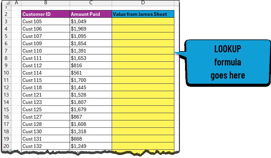
Example Formula: Suppose you have two sheets named “Sheet1” and “Sheet2.” In “Sheet1,” the Customer IDs are in column A, and the corresponding data you want to compare is in column B. In “Sheet2,” the Customer IDs are also in column A, and you want to retrieve the data from column B. Your VLOOKUP formula in the new worksheet would look like this:
=VLOOKUP(A2,Sheet2!$A$2:$B$100,2,FALSE)A2: The Customer ID in the current row of the new worksheet.Sheet2!$A$2:$B$100: The range in “Sheet2” that includes the Customer IDs and the data to retrieve. The$signs make the reference absolute, so it doesn’t change when you drag the formula down.2: The column number in thetable_array(Sheet2!$A$2:$B$100) from which to retrieve the data (column B).FALSE: Ensures an exact match for the Customer ID.
4.2. Understanding VLOOKUP Results
After entering the VLOOKUP formula, understanding the results is crucial for accurate comparison. VLOOKUP returns specific values based on whether it finds a match or not.
-
Matching Values:
- If VLOOKUP finds an exact match for the
lookup_valuein thetable_array, it returns the corresponding value from the specifiedcol_index_num. This indicates that the data in both sheets is identical for that particular unique identifier.
- If VLOOKUP finds an exact match for the
-
#N/A Error:
- If VLOOKUP cannot find a match for the
lookup_valuein thetable_array, it returns the#N/Aerror. This means that the unique identifier is missing in the second sheet. The#N/Aerror is a critical indicator of missing data.
- If VLOOKUP cannot find a match for the
-
Incorrect Values:
- If VLOOKUP returns a value that is different from what you expect, it could indicate a discrepancy between the two sheets. This could be due to data entry errors or differences in how the data was recorded.
-
Handling Errors:
-
To handle the
#N/Aerror, you can use theIFERRORfunction in Excel. This allows you to specify a custom value to return when VLOOKUP encounters an error. For example:=IFERROR(VLOOKUP(A2,Sheet2!$A$2:$B$100,2,FALSE), "Not Found")In this formula, if VLOOKUP returns
#N/A, the cell will display “Not Found” instead, making it easier to identify missing values.
-
4.3. Dragging the Formula Down
To apply the VLOOKUP formula to all rows in your new worksheet, you need to drag the formula down. This ensures that each row is compared and the results are displayed accordingly.
-
Select the Cell: Select the cell containing the VLOOKUP formula you just entered.
-
Locate the Fill Handle: Hover your mouse over the bottom-right corner of the selected cell. The cursor will change to a small black cross.
-
Drag Down: Click and drag the fill handle down to the last row of your data in the new worksheet. As you drag, the formula will automatically adjust to reference the correct rows.
-
Release the Mouse: Release the mouse button when you reach the last row. The VLOOKUP formula will be applied to all selected rows, and the results will be displayed in each cell.
-
Verify Results: Check the results in each row to ensure the formula is working correctly. Look for matching values,
#N/Aerrors, and any unexpected results.
4.4. Using Conditional Formatting to Highlight Differences
Conditional formatting can be used to automatically highlight differences between the two sheets, making it easier to spot discrepancies.
-
Select the Range: Select the range of cells in your new worksheet that contain the VLOOKUP results.
-
Open Conditional Formatting: Go to the “Home” tab in the Excel ribbon and click on “Conditional Formatting” in the “Styles” group.
-
Create a New Rule: Select “New Rule” from the dropdown menu.
-
Choose a Rule Type: In the “New Formatting Rule” dialog box, select “Use a formula to determine which cells to format.”
-
Enter the Formula: Enter a formula that identifies the differences you want to highlight. For example, to highlight cells where the VLOOKUP result is “#N/A,” you can use the following formula:
=ISNA(B2)B2: The first cell in the range you selected (adjust as necessary).ISNA: An Excel function that returns TRUE if the cell contains the#N/Aerror.
-
Set the Format: Click on the “Format” button to specify how you want the cells to be highlighted. You can change the fill color, font style, border, and more.
-
Click OK: Click “OK” to close the “Format Cells” dialog box, and then click “OK” again to close the “New Formatting Rule” dialog box.
-
Repeat for Other Conditions: Repeat these steps to create additional rules for other conditions, such as highlighting cells where the VLOOKUP result does not match the value in the first sheet.
By following this step-by-step guide, you can effectively use VLOOKUP to compare data between two Excel sheets, identify matches and differences, handle errors, and highlight discrepancies using conditional formatting.
5. Advanced VLOOKUP Techniques for Complex Comparisons
For more complex data comparisons, standard VLOOKUP may not suffice. This section explores advanced techniques to handle intricate scenarios and enhance your comparative analysis.
5.1. Using Multiple Criteria with VLOOKUP
Sometimes, a single unique identifier is not enough, and you need to use multiple criteria to accurately match records between two sheets. This can be achieved by creating a combined key column.
-
Create a Combined Key Column:
-
In both Excel sheets, insert a new column.
-
In the first row of the new column, enter a formula that concatenates the values from the columns you want to use as criteria. For example, if you want to combine “Customer ID” and “Product Code,” the formula might look like this:
=A2&"_"&B2A2: The cell containing the Customer ID.B2: The cell containing the Product Code.&"_"&: Concatenates the values with an underscore separator. You can use any separator that doesn’t appear in your data.
-
Drag the formula down to apply it to all rows.
-
-
Use the Combined Key in VLOOKUP:
-
In your new worksheet, set up the VLOOKUP formula using the combined key column as the
lookup_value. -
Ensure that the
table_arrayin the second sheet also includes the combined key column. -
The formula would look something like this:
=VLOOKUP(A2&"_"&B2,Sheet2!$C$2:$D$100,2,FALSE)A2&"_"&B2: Creates the combined key in the new worksheet.Sheet2!$C$2:$D$100: The range in “Sheet2” that includes the combined key column and the data to retrieve.
-
5.2. Handling Case Sensitivity
VLOOKUP is not case-sensitive by default, which can lead to inaccurate results if your data contains case variations. To handle case sensitivity, you can use a combination of VLOOKUP, EXACT, and IF functions.
-
Use the EXACT Function:
-
The
EXACTfunction compares two strings and returns TRUE if they are exactly the same, including case. -
In your new worksheet, create a new column and use the
EXACTfunction to compare thelookup_valuewith the values in the second sheet.=IF(EXACT(A2,INDEX(Sheet2!$A$2:$A$100,MATCH(A2,Sheet2!$A$2:$A$100,0))),VLOOKUP(A2,Sheet2!$A$2:$B$100,2,FALSE),"No Match")A2: Thelookup_valuein the current row of the new worksheet.INDEX(Sheet2!$A$2:$A$100,MATCH(A2,Sheet2!$A$2:$A$100,0)): Retrieves the corresponding value from the second sheet.VLOOKUP(A2,Sheet2!$A$2:$B$100,2,FALSE): Performs the VLOOKUP if theEXACTfunction returns TRUE."No Match": Returns “No Match” if theEXACTfunction returns FALSE.
-
5.3. Comparing Data with Fuzzy Matching
In some cases, you may need to compare data that is not exactly the same but similar. This is known as fuzzy matching. VLOOKUP is not designed for fuzzy matching, but you can use other techniques to achieve this.
-
Use the SOUNDEX Function:
-
The
SOUNDEXfunction converts a string to a four-character code based on how the string sounds. This can be useful for comparing names or words that are spelled differently but sound similar. -
In both Excel sheets, create a new column and use the
SOUNDEXfunction to generate the soundex code for the values you want to compare.=SOUNDEX(A2)A2: The cell containing the value you want to convert to a soundex code.
-
Use VLOOKUP to compare the soundex codes instead of the original values.
-
-
Use Third-Party Add-ins:
- Several third-party add-ins for Excel provide advanced fuzzy matching capabilities. These add-ins use algorithms to compare data based on similarity and can handle a wide range of scenarios.
5.4. Combining VLOOKUP with INDEX and MATCH
While VLOOKUP is useful, it has limitations. It can only look up values in the first column of the table_array and returns values from a specified column number. The INDEX and MATCH functions offer more flexibility.
-
The INDEX and MATCH Functions:
MATCH: Returns the position of a value in a range.INDEX: Returns the value at a specified position in a range.
-
Combining INDEX and MATCH:
-
You can use
INDEXandMATCHtogether to perform a lookup in any column and return values from any other column.=INDEX(Sheet2!$B$2:$B$100,MATCH(A2,Sheet2!$A$2:$A$100,0))Sheet2!$B$2:$B$100: The range containing the values you want to retrieve.A2: Thelookup_valuein the current row of the new worksheet.Sheet2!$A$2:$A$100: The range containing the values you want to match.
-
5.5. Using Power Query for Advanced Comparisons
Power Query is a powerful data transformation and analysis tool in Excel. It can be used to perform advanced comparisons between two or more sheets.
-
Load Data into Power Query:
- Go to the “Data” tab in the Excel ribbon and click on “From Table/Range.”
- Select the range of cells containing your data and click “OK.”
- Repeat this process for both Excel sheets.
-
Merge Queries:
- In the Power Query Editor, go to the “Home” tab and click on “Merge Queries.”
- Select the two queries you want to merge.
- Choose the columns you want to use as matching criteria.
- Select the type of join you want to perform (e.g., “Left Outer,” “Right Outer,” “Inner”).
- Click “OK.”
-
Expand Columns:
- After merging the queries, you can expand the columns from the second query to see the matching values.
- Click on the expand icon in the header of the merged column and select the columns you want to include.
- Click “OK.”
-
Load the Results:
- Go to the “Home” tab and click on “Close & Load” to load the results back into Excel.
By using these advanced VLOOKUP techniques, you can handle complex data comparisons, ensure accuracy, and gain deeper insights into your data.
6. Alternatives to VLOOKUP for Comparing Excel Sheets
While VLOOKUP is a popular choice for comparing data in Excel, several alternative methods offer unique advantages and may be more suitable for certain scenarios.
6.1. XLOOKUP
XLOOKUP is a more modern and versatile function than VLOOKUP. It addresses many of VLOOKUP’s limitations and offers improved functionality.
-
Advantages of XLOOKUP:
- Flexibility: XLOOKUP can look up values in any column and return values from any other column, without the need to specify a column number.
- Improved Syntax: XLOOKUP has a simpler and more intuitive syntax than VLOOKUP.
- Error Handling: XLOOKUP has built-in error handling, allowing you to specify a value to return if no match is found.
- Better Performance: XLOOKUP is generally faster and more efficient than VLOOKUP.
-
Using XLOOKUP:
-
The syntax for XLOOKUP is:
=XLOOKUP(lookup_value, lookup_array, return_array, [if_not_found], [match_mode], [search_mode])lookup_value: The value you want to search for.lookup_array: The range of cells where you want to search for thelookup_value.return_array: The range of cells containing the values you want to return.[if_not_found]: An optional argument that specifies the value to return if no match is found.[match_mode]: An optional argument that specifies the match mode (e.g., exact match, wildcard match).[search_mode]: An optional argument that specifies the search mode (e.g., search from first to last, search from last to first).
-
-
Example:
-
To compare data between two sheets using XLOOKUP, you can use the following formula:
=XLOOKUP(A2,Sheet2!$A$2:$A$100,Sheet2!$B$2:$B$100,"Not Found")A2: Thelookup_valuein the current row of the new worksheet.Sheet2!$A$2:$A$100: The range in “Sheet2” where you want to search for thelookup_value.Sheet2!$B$2:$B$100: The range in “Sheet2” containing the values you want to return."Not Found": The value to return if no match is found.
-
6.2. INDEX and MATCH
As mentioned earlier, the INDEX and MATCH functions can be used together as a more flexible alternative to VLOOKUP.
-
Advantages of INDEX and MATCH:
- Flexibility:
INDEXandMATCHcan look up values in any column and return values from any other column. - No Column Number: You don’t need to specify a column number, which can be error-prone.
- Dynamic:
INDEXandMATCHare more dynamic than VLOOKUP, as they adjust automatically if you insert or delete columns.
- Flexibility:
-
Using INDEX and MATCH:
-
The syntax for
INDEXandMATCHis:=INDEX(return_array, MATCH(lookup_value, lookup_array, 0))return_array: The range of cells containing the values you want to return.lookup_value: The value you want to search for.lookup_array: The range of cells where you want to search for thelookup_value.0: Specifies an exact match.
-
-
Example:
-
To compare data between two sheets using
INDEXandMATCH, you can use the following formula:=INDEX(Sheet2!$B$2:$B$100,MATCH(A2,Sheet2!$A$2:$A$100,0))Sheet2!$B$2:$B$100: The range in “Sheet2” containing the values you want to return.A2: Thelookup_valuein the current row of the new worksheet.Sheet2!$A$2:$A$100: The range in “Sheet2” where you want to search for thelookup_value.
-
6.3. Power Query
Power Query is a powerful data transformation and analysis tool in Excel that can be used to compare data between two or more sheets.
-
Advantages of Power Query:
- Advanced Transformations: Power Query allows you to perform a wide range of data transformations, such as merging, filtering, and aggregating.
- Multiple Data Sources: Power Query can connect to multiple data sources, including Excel files, databases, and web services.
- Automation: Power Query allows you to automate the data comparison process, so you can easily refresh the results when the data changes.
-
Using Power Query:
- Load Data: Load the data from both Excel sheets into Power Query.
- Merge Queries: Merge the queries based on a common column.
- Expand Columns: Expand the columns from the second query to see the matching values.
- Load Results: Load the results back into Excel.
6.4. Comparison Software
Dedicated comparison software offers advanced features and capabilities for comparing Excel sheets and other types of data.
-
Advantages of Comparison Software:
- Advanced Algorithms: Comparison software uses advanced algorithms to compare data based on similarity and can handle a wide range of scenarios.
- Detailed Reports: Comparison software generates detailed reports that highlight the differences between the two sheets.
- Automation: Comparison software allows you to automate the data comparison process.
-
Examples of Comparison Software:
- Diffchecker: A free online tool for comparing text files, images, and PDFs.
- Beyond Compare: A powerful comparison tool for Windows, macOS, and Linux.
- WinMerge: A free and open-source comparison tool for Windows.
By considering these alternatives to VLOOKUP, you can choose the method that best suits your needs and the complexity of your data comparison task.
7. Common Issues and Troubleshooting Tips for VLOOKUP
Even with careful setup, VLOOKUP can sometimes produce unexpected results. This section addresses common issues and provides troubleshooting tips to ensure accurate comparisons.
7.1. #N/A Errors
The #N/A error is one of the most common issues encountered when using VLOOKUP. It indicates that VLOOKUP could not find a match for the lookup_value in the table_array.
-
Causes of #N/A Errors:
- Missing Value: The
lookup_valueis not present in the first column of thetable_array. - Typos: There is a typographical error in the
lookup_valueor the values in thetable_array. - Incorrect Formatting: The
lookup_valueand the values in thetable_arrayhave different formatting (e.g., text vs. number). - Extra Spaces: There are extra spaces in the
lookup_valueor the values in thetable_array. - Case Sensitivity: VLOOKUP is not case-sensitive, but if you need to perform a case-sensitive comparison, you need to use a different approach.
- Missing Value: The
-
Troubleshooting Tips:
- Check for Missing Values: Ensure that the
lookup_valueis present in the first column of thetable_array. - Correct Typos: Carefully check for typographical errors in the
lookup_valueand the values in thetable_array. - Ensure Consistent Formatting: Ensure that the
lookup_valueand the values in thetable_arrayhave the same formatting (e.g., text, number, date). - Remove Extra Spaces: Use the
TRIMfunction to remove extra spaces from thelookup_valueand the values in thetable_array. - Use IFERROR: Use the
IFERRORfunction to handle the#N/Aerror and display a custom message.
- Check for Missing Values: Ensure that the
7.2. Incorrect Results
Sometimes, VLOOKUP may return a value, but it is not the value you expect. This can be due to several reasons.
-
Causes of Incorrect Results:
- Approximate Match: The
range_lookupargument is set to TRUE, which means VLOOKUP will return an approximate match. - Incorrect Column Number: The
col_index_numargument is incorrect, which means VLOOKUP is returning a value from the wrong column. - Duplicate Values: There are duplicate values in the first column of the
table_array, and VLOOKUP is returning the first match it finds. - Incorrect Table Array: The
table_arrayargument is incorrect, which means VLOOKUP is searching in the wrong range of cells.
- Approximate Match: The
-
Troubleshooting Tips:
- Use Exact Match: Set the
range_lookupargument to FALSE to ensure VLOOKUP returns an exact match. - Verify Column Number: Double-check the
col_index_numargument to ensure it is correct. - Remove Duplicates: Remove any duplicate values from the first column of the
table_array. - Verify Table Array: Double-check the
table_arrayargument to ensure it is correct.
- Use Exact Match: Set the
7.3. Performance Issues
VLOOKUP can be slow when working with large datasets. This can be due to several reasons.
-
Causes of Performance Issues:
- Large Datasets: VLOOKUP has to search through a large number of rows, which can take time.
- Volatile Functions: VLOOKUP is a volatile function, which means it recalculates every time the worksheet changes.
- Complex Formulas: Complex VLOOKUP formulas can take longer to calculate.
-
Troubleshooting Tips:
- Use XLOOKUP: XLOOKUP is generally faster and more efficient than VLOOKUP.
- Use INDEX and MATCH:
INDEXandMATCHcan be faster than VLOOKUP in some cases. - Optimize Formulas: Simplify your VLOOKUP formulas as much as possible.
- Use Helper Columns: Use helper columns to pre-calculate values that are used in VLOOKUP formulas.
- Disable Automatic Calculation: Disable automatic calculation and manually recalculate the worksheet when needed.
7.4. Case Sensitivity Issues
VLOOKUP is not case-sensitive, which can lead to incorrect results if your data contains case variations.
-
Causes of Case Sensitivity Issues:
- Case Variations: The
lookup_valueand the values in thetable_arrayhave different case (e.g., “Apple” vs. “apple”).
- Case Variations: The
-
Troubleshooting Tips:
- Use EXACT Function: Use the
EXACTfunction to perform a case-sensitive comparison. - Convert to Same Case: Convert all values to the same case using the
UPPERorLOWERfunctions.
- Use EXACT Function: Use the
7.5. Trailing Spaces
Trailing spaces can cause VLOOKUP to return incorrect results, as they are treated as part of the value.
-
Causes of Trailing Space Issues:
- Trailing Spaces: The
lookup_valueor the values in thetable_arrayhave trailing spaces.
- Trailing Spaces: The
-
Troubleshooting Tips:
- Use TRIM Function: Use the
TRIMfunction to remove trailing spaces from thelookup_valueand the values in thetable_array.
- Use TRIM Function: Use the
By addressing these common issues and following the troubleshooting tips, you can ensure that VLOOKUP returns accurate results and performs efficiently.
8. Optimizing Your Excel Sheets for Efficient VLOOKUP Comparisons
Optimizing your Excel sheets can significantly improve the efficiency and accuracy of VLOOKUP comparisons. This section provides tips for structuring your data, reducing file size, and using best practices to enhance performance.
8.1. Structuring Your Data Effectively
Proper data structuring is crucial for efficient VLOOKUP comparisons. A well-structured sheet ensures that VLOOKUP can quickly and accurately locate the required data.
-
Consistent Column Headers:
- Ensure that column headers are consistent across all sheets. Use the same names and formatting for identical columns.
-
Unique Identifiers:
- Use a unique identifier column to ensure that each row can be uniquely identified. This is essential for accurate VLOOKUP comparisons.
-
Data Types:
- Ensure that data types are consistent within each column. For example, if a column contains numbers, ensure that all values in that column are formatted as numbers.
-
Avoid Empty Rows and Columns:
- Remove any empty rows and columns that are not needed. Empty rows and columns can slow down VLOOKUP and make it more difficult to work with the data.
-
Use Tables:
- Convert your data ranges into Excel tables. Tables automatically adjust the range of cells used in formulas when you add or remove rows and columns.
8.2. Reducing File Size
Large Excel files can slow down VLOOKUP and make it more difficult to work with the data. Reducing file size can significantly improve performance.
-
Remove Unnecessary Data:
- Remove any data that is not needed for the comparison. This can include old data, summary data, and unused columns.
-
Compress Images:
- Compress any images in your Excel file to reduce their file size. You can do this by selecting the image, going to the “Format” tab, and clicking on “Compress Pictures.”
-
Save as .xlsx:
- Save your Excel file as a .xlsx file instead of a .xls file. The .xlsx format is more efficient and can significantly reduce file size.
-
Remove Formatting:
- Remove any unnecessary formatting from your Excel file. This can include excessive use of colors, fonts, and borders.
-
Use Helper Columns Sparingly:
- Use helper columns only when necessary. Excessive use of helper columns can increase file size and slow down performance.
8.3. Using Best Practices for VLOOKUP Formulas
Using best practices for VLOOKUP formulas can significantly improve their efficiency and accuracy.
-
Use Exact Match:
- Always use exact match (FALSE) in your VLOOKUP formulas unless you specifically need an approximate match.
-
Use Absolute References:
- Use absolute references ($) in your VLOOKUP formulas to prevent the table array from changing when you copy the formula.
-
Use Named Ranges:
- Use named ranges to make your VLOOKUP formulas more readable and easier to maintain.
-
Avoid Volatile Functions:
- Avoid using volatile functions in your VLOOKUP formulas. Volatile functions recalculate every time the worksheet changes, which can slow down performance.
-
Test Your Formulas:
- Test your VLOOKUP formulas thoroughly to ensure they are working correctly.
8.4. Leveraging Excel Features for Data Management
Excel offers several features that can help you manage your data more effectively and improve VLOOKUP performance.
-
Filters:
- Use filters to quickly find and compare data in your Excel sheets.
-
Sorting:
- Sort your data to make it easier to find and compare values.
3