When working with spreadsheets, comparing two columns to identify matches, differences, or missing data is a common task. VLOOKUP, a powerful Excel function, offers a versatile solution for this. This tutorial provides a comprehensive guide on how to leverage VLOOKUP for various column comparison scenarios.
Understanding VLOOKUP for Column Comparison
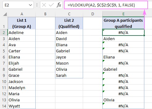
VLOOKUP (Vertical Lookup) searches for a specific value in the first column of a range and returns a corresponding value in the same row from a specified column. In the context of comparing two columns, VLOOKUP helps determine if values from one column exist in another.
Basic VLOOKUP Formula for Comparing Two Columns
The fundamental VLOOKUP formula for comparing two columns is:
=VLOOKUP(lookup_value, table_array, col_index_num, [range_lookup])- lookup_value: The value you want to find in the first column of the
table_array. Typically, this is a cell reference from the first column you’re comparing. - table_array: The range containing the data you want to search, including the column containing the
lookup_valueand the column from which you want to return a value. - col_index_num: The column number in the
table_arrayfrom which you want to retrieve the matching value. If you’re only checking for existence, this can be 1 (the same column as thelookup_value). - [range_lookup]: Set to
FALSEfor an exact match. This is crucial for accurate comparisons.
Handling #N/A Errors
When VLOOKUP doesn’t find a match, it returns a #N/A error. To make the results cleaner, use IFNA:
=IFNA(VLOOKUP(A2, $C$2:$C$9, 1, FALSE), "") This replaces errors with blank cells. You can customize the returned value:
=IFNA(VLOOKUP(A2, $C$2:$C$9, 1, FALSE), "Not Found")Comparing Columns Across Different Sheets
To compare columns on different sheets, include the sheet name in the table_array:
=IFNA(VLOOKUP(A2, Sheet2!$A$2:$A$9, 1, FALSE), "")Isolating Matches and Differences
Finding Common Values
To extract only the common values, filter the results of the basic VLOOKUP formula to remove blank cells or use the FILTER function in newer Excel versions:
=FILTER(A2:A14, IFNA(VLOOKUP(A2:A14, C2:C9, 1, FALSE), "")<>"")Finding Missing Values (Differences)
To identify values present in the first column but missing in the second, use ISNA with VLOOKUP:
=FILTER(A2:A14, ISNA(VLOOKUP(A2:A14, C2:C9, 1, FALSE)))Returning Values from a Third Column
VLOOKUP’s core strength is returning associated data. To compare two columns and retrieve a corresponding value from a third column:
=IFNA(VLOOKUP(A3, $D$3:$E$10, 2, FALSE), "")Here, col_index_num is 2, indicating the second column in the table_array (column E).
Conclusion
VLOOKUP is a highly effective tool for comparing two columns in Excel. By understanding its core functionality and combining it with other functions like IFNA, ISNA, and FILTER, you can perform comprehensive data comparisons to identify matches, differences, and extract associated information. Mastering VLOOKUP significantly enhances your spreadsheet analysis capabilities.