Comparing data across two Excel columns is a common task. Whether you’re identifying matches, finding discrepancies, or extracting corresponding values, VLOOKUP is a powerful tool. This tutorial provides a comprehensive guide on how to leverage VLOOKUP for various column comparison scenarios in Excel.
Understanding VLOOKUP for Column Comparison
VLOOKUP (Vertical Lookup) searches for a specific value in the first column of a range and returns a value in the same row from a specified column. For column comparison, we use VLOOKUP to check if values in one column exist in another.
Basic VLOOKUP Formula for Comparing Two Columns
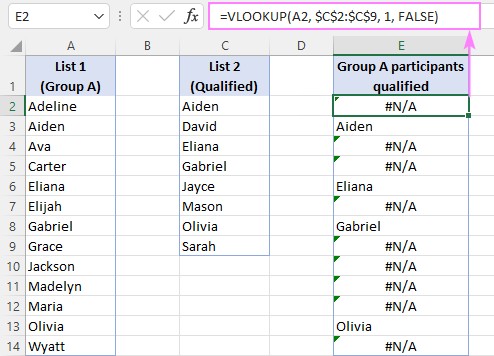
The fundamental VLOOKUP formula for comparing two columns (List 1 in column A and List 2 in column C) is:
=VLOOKUP(A2, $C$2:$C$9, 1, FALSE)Let’s break it down:
- A2: The lookup_value – the value you want to find in List 2.
- $C$2:$C$9: The table_array – the range containing List 2 (use absolute references “$” to keep the range fixed when copying the formula).
- 1: The col_index_num – since List 2 is in the first column of the table_array, we use 1.
- FALSE: The range_lookup – ensures an exact match.
This formula returns the matched value from List 2 if found in List 1. If not found, it returns an #N/A error.
Handling #N/A Errors
To replace #N/A errors with blank cells or custom text, use IFNA or IFERROR:
=IFNA(VLOOKUP(A2, $C$2:$C$9, 1, FALSE), "") // Blank cell
=IFNA(VLOOKUP(A2, $C$2:$C$9, 1, FALSE), "Not Found") // Custom text
Comparing Columns in Different Sheets
To compare columns across different sheets, include the sheet name in the table_array:
=IFNA(VLOOKUP(A2, Sheet2!$A$2:$A$9, 1, FALSE), "")Returning Common Values (Matches)
To extract only the common values, filter the results of the basic VLOOKUP formula to remove blank cells or use the FILTER function in Excel 365 and Excel 2021:
=FILTER(A2:A14, IFNA(VLOOKUP(A2:A14, C2:C9, 1, FALSE), "")<>"")Finding Missing Values (Differences)
To identify values present in List 1 but missing in List 2, use ISNA with VLOOKUP:
=IF(ISNA(VLOOKUP(A2, $C$2:$C$9, 1, FALSE)), A2, "")For dynamic filtering in Excel 365 and 2021:
=FILTER(A2:A14, ISNA(VLOOKUP(A2:A14, C2:C9, 1, FALSE)))Identifying Matches and Differences with Labels
To label each item in List 1 as “Found” or “Not Found” in List 2:
=IF(ISNA(VLOOKUP(A2, $D$2:$D$9, 1, FALSE)), "Not Found", "Found")Returning Values from a Third Column
To return a corresponding value from a third column (e.g., column E) based on matches between List 1 (column A) and List 2 (Column D):
=IFNA(VLOOKUP(A3, $D$3:$E$10, 2, FALSE), "")Conclusion
VLOOKUP offers a versatile way to compare two columns in Excel. By understanding its core functionality and combining it with other functions like IFNA, IFERROR, and FILTER, you can efficiently analyze and manipulate data for various comparison tasks. This tutorial has equipped you with the knowledge to effectively utilize VLOOKUP for comprehensive column comparisons in Excel.