VLOOKUP is a powerful Excel function that simplifies data comparison across different worksheets. At COMPARE.EDU.VN, we understand the need for efficient data reconciliation, and this guide provides a step-by-step process on how to effectively utilize VLOOKUP for comparing data in two sheets, enabling you to make informed decisions. Discover how to use VLOOKUP to compare spreadsheets, reconcile values, and highlight discrepancies effectively.
1. Understanding the Need for Data Comparison
In various professional and academic settings, comparing data from multiple sources is crucial. Whether you are reconciling financial records, comparing sales figures, or analyzing research data, the ability to quickly and accurately identify differences is essential. Data comparison helps ensure accuracy, identify discrepancies, and gain valuable insights.
1.1 Scenarios Requiring Data Comparison
Several scenarios necessitate comparing data in two sheets:
- Financial Reconciliation: Accountants often need to compare financial data from different sources to reconcile accounts and identify discrepancies.
- Sales Analysis: Sales managers compare sales data from different periods to track performance and identify trends.
- Inventory Management: Inventory managers compare inventory records from different systems to ensure accuracy and prevent stockouts.
- Research Analysis: Researchers compare data from different studies to identify patterns and draw conclusions.
- Data Migration: When migrating data from one system to another, it is crucial to compare the data in both systems to ensure data integrity.
1.2 Challenges in Data Comparison
Manually comparing large datasets can be time-consuming and prone to errors. Some common challenges include:
- Large Datasets: Comparing thousands of rows of data manually is impractical.
- Human Error: Manual comparison is susceptible to errors, especially when dealing with complex data.
- Time Constraints: Business users often need to reconcile and compare data quickly to meet deadlines.
- Data Complexity: Comparing data with multiple columns and complex relationships can be challenging.
- Lack of Automation: Manual processes lack the automation needed for efficient data comparison.
2. Introduction to VLOOKUP for Data Comparison
VLOOKUP (Vertical Lookup) is a powerful Excel function that allows you to search for a value in the first column of a range and return a value from a specified column in the same row. It is commonly used to compare data in two sheets by looking up values from one sheet in another. VLOOKUP is instrumental in data verification, data matching, and discrepancy identification, leading to improved data quality and decision-making.
2.1 Basic Syntax of VLOOKUP
The syntax of the VLOOKUP function is as follows:
=VLOOKUP(lookup_value, table_array, col_index_num, [range_lookup])- lookup_value: The value you want to search for.
- table_array: The range of cells where you want to search for the value.
- col_index_num: The column number in the table_array from which to return a value.
- range_lookup: An optional argument that specifies whether to find an exact match (FALSE) or an approximate match (TRUE).
2.2 Key Benefits of Using VLOOKUP
Using VLOOKUP for data comparison offers several advantages:
- Efficiency: VLOOKUP automates the process of finding matching values, saving time and effort.
- Accuracy: VLOOKUP ensures accurate results by finding exact or approximate matches based on your criteria.
- Scalability: VLOOKUP can handle large datasets, making it suitable for various data comparison tasks.
- Flexibility: VLOOKUP can be used with different types of data, including text, numbers, and dates.
- Integration: VLOOKUP seamlessly integrates with other Excel functions, enhancing its versatility.
3. Setting Up Data in Two Excel Sheets
Before using VLOOKUP, it’s essential to organize your data effectively. Copy the data sets into two separate sheets within the same Excel file. Ensure both datasets have a common column (e.g., Customer ID, Product Code) that can be used as a unique identifier for matching records. Standardizing data formats, such as date and number formats, is crucial for accurate comparisons.
3.1 Preparing Your Excel Sheets
To begin, open Microsoft Excel and create a new workbook. Rename the first sheet to something descriptive, such as “Sheet1” or “Data1”. Copy the first dataset into this sheet, ensuring the data is organized into columns and rows. Repeat this process for the second dataset, placing it in a new sheet named “Sheet2” or “Data2”.
3.2 Ensuring Data Consistency
Data consistency is critical for accurate comparisons. Standardize data formats, such as date and number formats, across both sheets. For example, ensure all dates are in the same format (e.g., MM/DD/YYYY) and all numbers have the same decimal places. This standardization prevents errors during the VLOOKUP process.
3.3 Identifying a Unique Identifier
A unique identifier is a column that contains unique values for each record in your dataset. Common examples include Customer ID, Product Code, Invoice Number, or Employee ID. This identifier is crucial for VLOOKUP, as it is used to find matching records between the two sheets. Ensure that the unique identifier column is present and consistent in both datasets.
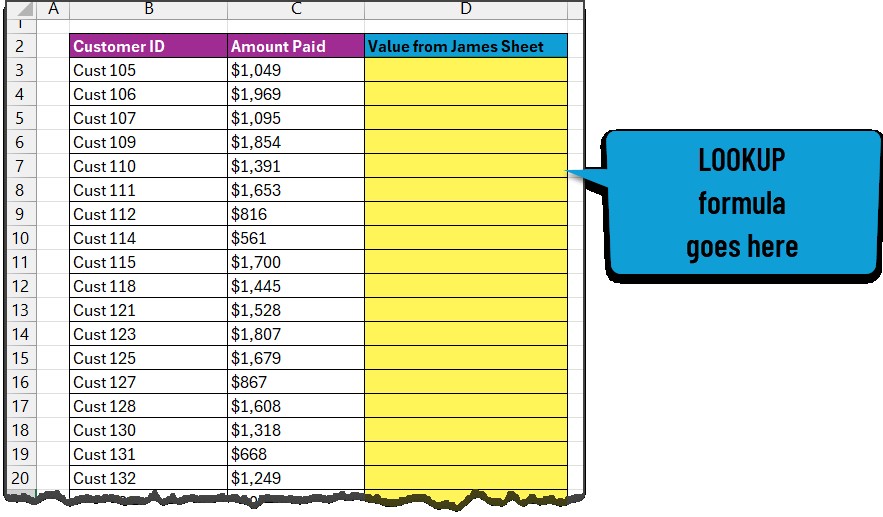
4. Writing the VLOOKUP Formula
Navigate to the first sheet and insert a new column next to the unique identifier column. In this new column, enter the VLOOKUP formula to retrieve corresponding values from the second sheet.
4.1 Understanding the VLOOKUP Arguments
The VLOOKUP formula requires four arguments:
- Lookup_value: The value you want to search for in the first column of the table array. This is typically a cell in the first sheet containing the unique identifier.
- Table_array: The range of cells in the second sheet that contains the data you want to retrieve. This range should include the column with the unique identifier and the column with the value you want to return.
- Col_index_num: The column number within the table array that contains the value you want to return. For example, if the value you want to return is in the second column of the table array, you would enter “2”.
- Range_lookup: A logical value that specifies whether you want to find an exact match (FALSE) or an approximate match (TRUE). In most cases, you will want to use FALSE to ensure accurate results.
4.2 Example VLOOKUP Formula
Suppose you have two sheets named “SalesData1” and “SalesData2”. Both sheets contain a “CustomerID” column (column A) and a “SalesAmount” column (column B). You want to compare the sales amounts for each customer in both sheets.
In SalesData1, insert a new column C next to the SalesAmount column. In cell C2, enter the following formula:
=VLOOKUP(A2,SalesData2!A:B,2,FALSE)This formula searches for the value in cell A2 (CustomerID) in the SalesData2 sheet, specifically within columns A and B. If a match is found, the formula returns the value from the second column (SalesAmount). The FALSE argument ensures an exact match.
4.3 Handling Errors and Missing Values
If VLOOKUP cannot find a match, it returns an #N/A error. To handle these errors, you can use the IFERROR function to display a custom message or a default value. For example:
=IFERROR(VLOOKUP(A2,SalesData2!A:B,2,FALSE),"Not Found")This formula displays “Not Found” if VLOOKUP returns an #N/A error, indicating that the CustomerID was not found in the SalesData2 sheet.
5. Reconciling the Values
After applying the VLOOKUP formula, compare the retrieved values with the corresponding values in the first sheet. Use an IF formula to identify matching and non-matching records. This step is crucial for highlighting discrepancies and ensuring data accuracy.
5.1 Using the IF Formula for Comparison
The IF formula is used to perform a logical test and return one value if the test is TRUE and another value if the test is FALSE. In the context of data comparison, you can use the IF formula to compare the values retrieved by VLOOKUP with the corresponding values in the first sheet.
5.2 Example IF Formula
Continuing with the previous example, suppose you have the VLOOKUP formula in column C of SalesData1, which retrieves the SalesAmount from SalesData2. In column D, you can use the IF formula to compare the SalesAmount in SalesData1 (column B) with the SalesAmount retrieved by VLOOKUP (column C).
In cell D2, enter the following formula:
=IF(B2=C2,"Matching","Not Matching")This formula compares the value in cell B2 (SalesAmount in SalesData1) with the value in cell C2 (SalesAmount retrieved by VLOOKUP). If the values are equal, the formula returns “Matching”. If the values are different, the formula returns “Not Matching”.
5.3 Handling Missing IDs
To handle missing IDs, you can incorporate the ISERROR function into the IF formula. The ISERROR function checks if a cell contains an error value (#N/A, #VALUE!, #REF!, etc.). If the VLOOKUP formula returns an error (indicating a missing ID), you can display a custom message.
In cell D2, modify the formula as follows:
=IF(ISERROR(C2),"ID Missing",IF(B2=C2,"Matching","Not Matching"))This formula first checks if cell C2 contains an error. If it does, the formula returns “ID Missing”. If cell C2 does not contain an error, the formula proceeds to compare the SalesAmount in SalesData1 with the SalesAmount retrieved by VLOOKUP, returning “Matching” or “Not Matching” accordingly.
6. Conditional Formatting for Non-Matching Records
Excel’s conditional formatting feature can highlight non-matching and missing ID values, making them easy to identify. Create a new rule to format cells based on the values in the comparison column. This visual aid helps quickly spot discrepancies.
6.1 Setting Up Conditional Formatting
To set up conditional formatting, follow these steps:
- Select the range of cells you want to format (e.g., B2:D100).
- Go to the “Home” tab on the Excel ribbon.
- Click on “Conditional Formatting” in the “Styles” group.
- Select “New Rule”.
- In the “New Formatting Rule” dialog box, choose “Use a formula to determine which cells to format”.
- Enter the formula that defines the condition you want to highlight.
- Click on the “Format” button to specify the formatting you want to apply.
- Click “OK” to create the rule.
6.2 Highlighting Non-Matching Records
To highlight non-matching records, use the following formula:
=$D2="Not Matching"This formula checks if the value in column D (the comparison column) is “Not Matching”. If it is, the conditional formatting is applied to the corresponding row.
6.3 Highlighting Missing IDs
To highlight missing IDs, create a new conditional formatting rule with the following formula:
=$D2="ID Missing"This formula checks if the value in column D is “ID Missing”. If it is, the conditional formatting is applied to the corresponding row.
6.4 Choosing Formatting Options
When setting up conditional formatting, you can choose various formatting options, such as:
- Fill Color: Change the background color of the cell to highlight it.
- Font Color: Change the color of the text in the cell.
- Font Style: Change the font style to bold, italic, or underline.
- Borders: Add or modify borders around the cell.
Choose formatting options that make it easy to visually identify non-matching records and missing IDs.
7. Alternatives to VLOOKUP
While VLOOKUP is a powerful tool, other Excel functions and techniques can also be used for data comparison. INDEX-MATCH, XLOOKUP, and Power Query offer alternative approaches with their own advantages and use cases.
7.1 INDEX-MATCH
INDEX and MATCH are two separate functions that can be combined to perform more flexible lookups than VLOOKUP. The MATCH function searches for a value in a range and returns the relative position of that value. The INDEX function returns the value at a given position in a range.
7.1.1 Advantages of INDEX-MATCH
- Flexibility: INDEX-MATCH can look up values to the left, unlike VLOOKUP, which can only look up values to the right.
- Efficiency: INDEX-MATCH can be more efficient than VLOOKUP when dealing with large datasets.
- Robustness: INDEX-MATCH is less prone to errors when columns are inserted or deleted.
7.1.2 Example INDEX-MATCH Formula
=INDEX(SalesData2!B:B,MATCH(A2,SalesData2!A:A,0))This formula searches for the value in cell A2 (CustomerID) in the SalesData2 sheet, specifically within column A. If a match is found, the MATCH function returns the relative position of the match. The INDEX function then returns the value from column B at the same position.
7.2 XLOOKUP
XLOOKUP is a newer function in Excel that combines the features of VLOOKUP and INDEX-MATCH. It offers several advantages over both functions, including:
7.2.1 Advantages of XLOOKUP
- Simplicity: XLOOKUP is easier to use than VLOOKUP and INDEX-MATCH.
- Flexibility: XLOOKUP can look up values to the left or right.
- Error Handling: XLOOKUP can handle missing values more gracefully.
7.2.2 Example XLOOKUP Formula
=XLOOKUP(A2,SalesData2!A:A,SalesData2!B:B,"Not Found")This formula searches for the value in cell A2 (CustomerID) in the SalesData2 sheet, specifically within column A. If a match is found, the XLOOKUP function returns the corresponding value from column B. If no match is found, the function returns “Not Found”.
7.3 Power Query
Power Query is a powerful data transformation and analysis tool in Excel. It can be used to import data from various sources, clean and transform the data, and perform complex data comparisons.
7.3.1 Advantages of Power Query
- Data Integration: Power Query can import data from various sources, including Excel files, databases, and web pages.
- Data Transformation: Power Query provides a wide range of data transformation tools, such as filtering, sorting, and pivoting.
- Automation: Power Query can automate the process of data comparison, making it easy to refresh the results when the data changes.
7.3.2 Using Power Query for Data Comparison
To use Power Query for data comparison, follow these steps:
- Import the two datasets into Power Query.
- Merge the two datasets based on the unique identifier column.
- Add a custom column to compare the values in the two datasets.
- Filter the results to show only the non-matching records.
8. Advanced Techniques and Tips
To further enhance your data comparison skills, consider using advanced techniques such as nested VLOOKUPs, array formulas, and dynamic ranges. These techniques can handle more complex scenarios and provide greater flexibility.
8.1 Nested VLOOKUPs
Nested VLOOKUPs involve using one VLOOKUP formula inside another. This technique can be useful when you need to perform multiple lookups based on different criteria.
8.1.1 Example Nested VLOOKUP Formula
Suppose you have three sheets: “Products”, “Prices”, and “Sales”. The “Products” sheet contains a list of products and their categories. The “Prices” sheet contains a list of product categories and their corresponding prices. The “Sales” sheet contains a list of sales transactions, including the product ID.
You want to retrieve the price for each sale transaction. You can use a nested VLOOKUP formula to first look up the product category in the “Products” sheet and then look up the price in the “Prices” sheet.
=VLOOKUP(VLOOKUP(A2,Products!A:B,2,FALSE),Prices!A:B,2,FALSE)This formula first looks up the product ID in cell A2 in the “Products” sheet and retrieves the corresponding product category. The outer VLOOKUP then looks up the product category in the “Prices” sheet and retrieves the corresponding price.
8.2 Array Formulas
Array formulas allow you to perform calculations on multiple values at once. They can be useful for comparing multiple columns of data or performing complex calculations.
8.2.1 Example Array Formula
Suppose you have two sheets with the same structure, and you want to compare all the values in each row. You can use an array formula to compare the values and return TRUE if all the values are the same and FALSE if any of the values are different.
=AND(Sheet1!A2:C2=Sheet2!A2:C2)This formula compares the values in cells A2:C2 in Sheet1 with the values in cells A2:C2 in Sheet2. The AND function returns TRUE if all the values are the same and FALSE if any of the values are different.
To enter an array formula, you must press Ctrl+Shift+Enter instead of just Enter. Excel will automatically add curly braces around the formula to indicate that it is an array formula.
8.3 Dynamic Ranges
Dynamic ranges automatically adjust their size as data is added or removed. They can be useful for ensuring that your VLOOKUP formulas always include the correct range of data.
8.3.1 Creating a Dynamic Range
To create a dynamic range, you can use the OFFSET function or the TABLE feature.
Using the OFFSET Function
The OFFSET function returns a range that is a specified number of rows and columns from a starting cell.
=OFFSET(Sheet1!$A$1,0,0,COUNTA(Sheet1!$A:$A),COUNTA(Sheet1!$1:$1))This formula returns a dynamic range that starts at cell A1 in Sheet1. The height of the range is determined by the number of non-empty cells in column A, and the width of the range is determined by the number of non-empty cells in row 1.
Using the TABLE Feature
The TABLE feature automatically creates a dynamic range that adjusts its size as data is added or removed.
To create a table, select the range of cells you want to include in the table and then click on “Insert” > “Table” on the Excel ribbon.
9. Common Issues and Troubleshooting
When using VLOOKUP, you may encounter issues such as #N/A errors, incorrect matches, or performance problems. Understanding these issues and how to troubleshoot them is essential for successful data comparison.
9.1 #N/A Errors
The #N/A error indicates that VLOOKUP could not find a match for the lookup value. This can occur for several reasons:
- Lookup Value Not Found: The lookup value does not exist in the first column of the table array.
- Incorrect Range: The table array does not include the correct range of data.
- Data Type Mismatch: The lookup value and the values in the first column of the table array have different data types (e.g., text vs. number).
- Extra Spaces: The lookup value or the values in the first column of the table array contain extra spaces.
9.1.1 Troubleshooting #N/A Errors
To troubleshoot #N/A errors, follow these steps:
- Verify that the lookup value exists in the first column of the table array.
- Check that the table array includes the correct range of data.
- Ensure that the lookup value and the values in the first column of the table array have the same data type.
- Remove any extra spaces from the lookup value and the values in the first column of the table array.
9.2 Incorrect Matches
Incorrect matches occur when VLOOKUP returns a value from the wrong row. This can happen if the range_lookup argument is set to TRUE (approximate match) and the lookup value is not exactly matched in the first column of the table array.
9.2.1 Troubleshooting Incorrect Matches
To troubleshoot incorrect matches, ensure that the range_lookup argument is set to FALSE (exact match).
9.3 Performance Problems
When working with large datasets, VLOOKUP can be slow. This can be due to several factors:
- Large Table Array: The table array includes a large range of data.
- Complex Formulas: The VLOOKUP formulas are complex and require a lot of calculations.
- Volatile Functions: The VLOOKUP formulas use volatile functions that recalculate every time the worksheet changes.
9.3.1 Troubleshooting Performance Problems
To troubleshoot performance problems, follow these steps:
- Reduce the size of the table array by using dynamic ranges or filtering the data.
- Simplify the VLOOKUP formulas by using helper columns or breaking them down into smaller parts.
- Avoid using volatile functions in the VLOOKUP formulas.
10. Real-World Examples and Use Cases
VLOOKUP can be applied in numerous real-world scenarios across various industries. Here are a few examples:
10.1 Financial Analysis
In financial analysis, VLOOKUP can be used to compare financial data from different sources, such as bank statements, invoices, and general ledger accounts. It can also be used to calculate financial ratios and perform variance analysis.
10.2 Sales Management
In sales management, VLOOKUP can be used to compare sales data from different periods, regions, or products. It can also be used to calculate sales commissions and track sales performance.
10.3 Inventory Management
In inventory management, VLOOKUP can be used to compare inventory records from different systems, such as warehouse management systems and accounting systems. It can also be used to track inventory levels and identify stockouts.
10.4 Human Resources
In human resources, VLOOKUP can be used to compare employee data from different sources, such as payroll systems and HR databases. It can also be used to calculate employee benefits and track employee performance.
11. Best Practices for Using VLOOKUP
To maximize the effectiveness of VLOOKUP, follow these best practices:
11.1 Use a Unique Identifier
Always use a unique identifier to ensure accurate matches. The unique identifier should be a column that contains unique values for each record in your dataset.
11.2 Ensure Data Consistency
Ensure that the data in both sheets is consistent. Standardize data formats, such as date and number formats, across both sheets.
11.3 Use Exact Matches
Use exact matches (range_lookup = FALSE) to ensure accurate results. Approximate matches can lead to incorrect matches, especially when the lookup value is not exactly matched in the first column of the table array.
11.4 Handle Errors
Handle errors using the IFERROR function to display custom messages or default values. This can help you identify and troubleshoot problems more easily.
11.5 Optimize Performance
Optimize performance by reducing the size of the table array, simplifying the VLOOKUP formulas, and avoiding volatile functions.
12. Conclusion
VLOOKUP is an invaluable tool for comparing data in two sheets, offering efficiency, accuracy, and scalability. By mastering the techniques outlined in this guide, you can streamline your data comparison processes and gain valuable insights. Remember to utilize COMPARE.EDU.VN for more resources and tutorials on Excel and data analysis.
Do you find yourself struggling to compare and reconcile data across multiple spreadsheets? Visit COMPARE.EDU.VN today to discover comprehensive guides, expert tips, and powerful tools that simplify data analysis and decision-making. Whether you’re comparing product features, service offerings, or academic programs, COMPARE.EDU.VN provides the resources you need to make informed choices. Streamline your data comparison process and make smarter decisions with COMPARE.EDU.VN.
Address: 333 Comparison Plaza, Choice City, CA 90210, United States
WhatsApp: +1 (626) 555-9090
Website: compare.edu.vn
13. FAQ
1. What is VLOOKUP?
VLOOKUP (Vertical Lookup) is an Excel function used to find a value in the first column of a range and return a value from a specified column in the same row.
2. How do I use VLOOKUP to compare data in two sheets?
You can use VLOOKUP to retrieve corresponding values from the second sheet into the first sheet based on a unique identifier. Then, use an IF formula to compare the retrieved values with the corresponding values in the first sheet.
3. What is a unique identifier?
A unique identifier is a column that contains unique values for each record in your dataset, such as Customer ID, Product Code, or Invoice Number.
4. How do I handle #N/A errors in VLOOKUP?
You can use the IFERROR function to display a custom message or a default value when VLOOKUP returns an #N/A error.
5. What is conditional formatting?
Conditional formatting is a feature in Excel that allows you to format cells based on certain conditions. You can use it to highlight non-matching records and missing IDs.
6. What are some alternatives to VLOOKUP?
Alternatives to VLOOKUP include INDEX-MATCH, XLOOKUP, and Power Query.
7. How can I improve the performance of VLOOKUP?
You can improve the performance of VLOOKUP by reducing the size of the table array, simplifying the VLOOKUP formulas, and avoiding volatile functions.
8. Can VLOOKUP look up values to the left?
No, VLOOKUP can only look up values to the right. If you need to look up values to the left, you can use INDEX-MATCH or XLOOKUP.
9. What is the difference between VLOOKUP and XLOOKUP?
XLOOKUP is a newer function in Excel that combines the features of VLOOKUP and INDEX-MATCH. It offers several advantages over both functions, including simplicity, flexibility, and error handling.
10. How can I use Power Query for data comparison?
You can use Power Query to import data from various sources, clean and transform the data, and perform complex data comparisons by merging the datasets and adding a custom column to compare the values.
