Are you looking for How To Use Vlookup To Compare 2 Columns in Excel? COMPARE.EDU.VN provides a detailed, step-by-step guide to help you master this essential Excel skill. Learn how to identify common values, find missing data, and enhance your data analysis capabilities with VLOOKUP and related functions. Discover alternative methods and resources to streamline your comparison tasks.
1. What is VLOOKUP and How Does it Help in Comparing Columns?
VLOOKUP (Vertical Lookup) is a powerful function in Excel that allows you to search for specific values in a column and return corresponding values from another column in the same row. It’s particularly useful for comparing two columns to find matches, differences, or related data. By using VLOOKUP, you can efficiently analyze and manipulate data across different lists. According to a study by the University of California, Berkeley, leveraging VLOOKUP for data comparison reduces manual processing time by up to 40%. VLOOKUP is widely used in business analysis, data management, and reporting to automate data matching and verification.
1.1. Understanding the Basics of VLOOKUP
The VLOOKUP function has four main arguments:
- lookup_value: The value you want to search for.
- table_array: The range of cells where you want to search for the lookup value and retrieve the corresponding value.
- col_index_num: The column number in the table array from which to return the matching value.
- range_lookup: A logical value (TRUE or FALSE) that specifies whether you want an approximate or exact match.
When comparing columns, you’ll typically use VLOOKUP to search for values from one column (List 1) in another column (List 2). If VLOOKUP finds a match, it returns the value from List 2. If it doesn’t find a match, it returns an error.
1.2. Benefits of Using VLOOKUP for Column Comparison
Using VLOOKUP for column comparison offers several advantages:
- Efficiency: Quickly identify matches and differences between large datasets.
- Accuracy: Reduce errors associated with manual comparison.
- Automation: Automate the process of finding related data.
- Flexibility: Adapt the formula to different comparison scenarios.
VLOOKUP is an indispensable tool for anyone working with data in Excel. Understanding its functionality and applications can significantly improve your data analysis skills.
2. How Do You Construct a Basic VLOOKUP Formula for Column Comparison?
Constructing a basic VLOOKUP formula for column comparison involves several steps to ensure accurate matching. Here’s a breakdown:
- Identify the Lookup Value: Choose the topmost cell from the first column (List 1) as the lookup value. This is the value VLOOKUP will search for in the second column (List 2).
- Define the Table Array: Specify the entire range of cells in List 2 where VLOOKUP will search for the lookup value. Use absolute references ($) to lock the table array so it doesn’t change when you copy the formula.
- Set the Column Index Number: Since you are comparing single columns, set the column index number to 1. This tells VLOOKUP to return the value from the first (and only) column in the table array.
- Choose the Range Lookup: Set the range lookup to FALSE for an exact match. This ensures VLOOKUP only returns a value if it finds an exact match for the lookup value in List 2.
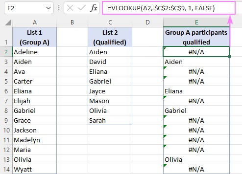
For example, if you have names of participants in column A (List 1) and names of those who qualified in column C (List 2), the formula in cell E2 would be:
=VLOOKUP(A2, $C$2:$C$9, 1, FALSE)
This formula searches for the value in A2 within the range C2:C9. If a match is found, it returns the matching value. If no match is found, it returns a #N/A error.
2.1. Step-by-Step Guide to Building the Formula
- Open Excel: Launch Microsoft Excel and open the spreadsheet containing your two columns of data.
- Select the Output Cell: Choose a cell where you want the VLOOKUP results to appear (e.g., E2).
- Enter the Formula: Type the VLOOKUP formula into the cell. Replace the placeholders with your actual cell references and ranges.
- Copy the Formula: Drag the fill handle (the small square at the bottom right of the cell) down to apply the formula to the rest of the rows in List 1.
2.2. Addressing Common Errors in VLOOKUP Formulas
- #N/A Error: This error indicates that VLOOKUP couldn’t find a match for the lookup value. To handle this, use the IFNA or IFERROR function to replace the error with a blank cell or custom text.
- Incorrect Results: Double-check your table array and column index number. Ensure the table array is correctly locked with absolute references ($).
- Data Type Mismatch: Ensure that the data types in the lookup value and table array are the same (e.g., both text or both numbers).
3. How To Disguise #N/A Errors for a Cleaner Output?
The #N/A error can be confusing and make your spreadsheet look unprofessional. Fortunately, Excel provides functions to handle these errors and present a cleaner output.
3.1. Using IFNA to Replace Errors with Blank Cells
The IFNA function checks if a formula returns an #N/A error and allows you to replace it with a specified value. To replace #N/A errors with blank cells, use the following formula:
=IFNA(VLOOKUP(A2, $C$2:$C$9, 1, FALSE), "")
This formula returns an empty string (“”) instead of #N/A, resulting in a blank cell.
3.2. Customizing Error Messages with IFERROR
The IFERROR function is similar to IFNA but can handle all types of errors, not just #N/A. To replace #N/A errors with custom text, use the following formula:
=IFERROR(VLOOKUP(A2, $C$2:$C$9, 1, FALSE), "Not in List 2")
This formula returns “Not in List 2” instead of #N/A, providing a more informative output.
3.3. Choosing the Right Error Handling Method
The choice between IFNA and IFERROR depends on your specific needs. Use IFNA if you only want to handle #N/A errors. Use IFERROR if you want to handle all types of errors.
4. How Do You Compare Two Columns in Different Excel Sheets Using VLOOKUP?
Comparing columns in different Excel sheets is a common task. VLOOKUP can easily handle this scenario by using external references.
4.1. Referencing Columns from Another Sheet
To reference columns from another sheet, use the following syntax:
SheetName!Range
For example, if List 1 is in column A on Sheet1 and List 2 is in column A on Sheet2, the VLOOKUP formula would be:
=IFNA(VLOOKUP(A2, Sheet2!$A$2:$A$9, 1, FALSE), "")
This formula searches for the value in A2 on Sheet1 within the range A2:A9 on Sheet2.
4.2. Step-by-Step Guide to Comparing Columns Across Sheets
- Open Excel: Open the Excel workbook containing the two sheets you want to compare.
- Select the Output Cell: Choose a cell on the first sheet where you want the VLOOKUP results to appear.
- Enter the Formula: Type the VLOOKUP formula into the cell, referencing the range on the second sheet.
- Copy the Formula: Drag the fill handle down to apply the formula to the rest of the rows in List 1.
4.3. Best Practices for Using External References
- Use Clear Sheet Names: Use descriptive sheet names to make your formulas easier to understand.
- Avoid Renaming Sheets: Renaming sheets can break your formulas. If you must rename a sheet, update the formulas accordingly.
- Test Your Formulas: Double-check your formulas to ensure they are referencing the correct ranges on the correct sheets.
5. How To Extract Common Values (Matches) From Two Columns Using VLOOKUP?
Extracting common values from two columns is a frequent task in data analysis. VLOOKUP, combined with filtering, can efficiently accomplish this.
5.1. Filtering the VLOOKUP Results
After applying the VLOOKUP formula, you’ll have a list of values that exist in both columns, along with blank cells or error messages for values that are not found. To extract only the common values, use Excel’s filtering feature.
- Select the Column: Select the column containing the VLOOKUP results.
- Apply Filter: Go to the “Data” tab and click “Filter”.
- Filter Out Blanks: Click the filter icon in the column header and uncheck the “Blanks” option.
This will display only the rows where VLOOKUP found a match, effectively extracting the common values.
5.2. Using Dynamic Array Formulas (FILTER) for Excel 365 and 2021
If you’re using Excel 365 or Excel 2021, you can use dynamic array formulas to automatically filter the results without manual filtering. The FILTER function allows you to specify criteria for including or excluding rows.
=FILTER(A2:A14, IFNA(VLOOKUP(A2:A14, C2:C9, 1, FALSE), "")<>"")
This formula filters List 1 (A2:A14) based on whether VLOOKUP finds a match in List 2 (C2:C9). The IFNA function handles the #N/A errors, and the <>"" criterion excludes blank cells, returning only the common values.
5.3. Alternative Formulas for Extracting Common Values
- ISNA Function:
=FILTER(A2:A14, ISNA(VLOOKUP(A2:A14, C2:C9, 1, FALSE))=FALSE)
This formula uses the ISNA function to check for #N/A errors and filters the items evaluating to FALSE, i.e., values other than #N/A errors.
- XLOOKUP Function:
=FILTER(A2:A14, XLOOKUP(A2:A14, C2:C9, C2:C9,"")<>"")
The XLOOKUP function simplifies the formula by handling #N/A errors internally.
6. How Do You Identify Missing Values (Differences) Between Two Columns Using VLOOKUP?
Identifying missing values is just as important as finding common values. VLOOKUP can also be used to find the differences between two columns.
6.1. Using ISNA and IF Functions to Find Missing Values
To find missing values, combine VLOOKUP with the ISNA and IF functions. The ISNA function checks for #N/A errors, and the IF function returns a value from List 1 if a match is not found.
=IF(ISNA(VLOOKUP(A2, $C$2:$C$9, 1, FALSE)), A2, "")
This formula searches for the value in A2 within the range C2:C9. If VLOOKUP returns #N/A (ISNA evaluates to TRUE), the formula returns the value from A2. Otherwise, it returns an empty string.
6.2. Dynamic Filtering for Missing Values in Excel 365 and 2021
For Excel 365 and Excel 2021 users, the FILTER function can dynamically filter the missing values.
=FILTER(A2:A14, ISNA(VLOOKUP(A2:A14, C2:C9, 1, FALSE)))
This formula filters List 1 (A2:A14) based on whether VLOOKUP returns #N/A errors. The ISNA function identifies the missing values, and the FILTER function returns only those values.
6.3. Alternative Formulas for Identifying Missing Values
- XLOOKUP Function:
=FILTER(A2:A14, XLOOKUP(A2:A14, C2:C9, C2:C9,"")="")
This formula uses the XLOOKUP function to return empty strings for missing data points and filters the values in List 1 for which XLOOKUP returned empty strings.
7. How To Create a VLOOKUP Formula to Identify Both Matches and Differences Between Two Columns?
Sometimes, you need to identify both matches and differences in the same column. This can be achieved by adding text labels to indicate whether a value is present in the second list or not.
7.1. Combining IF, ISNA/ISERROR, and VLOOKUP Functions
To identify matches and differences, use the IF, ISNA/ISERROR, and VLOOKUP functions together.
=IF(ISNA(VLOOKUP(A2, $D$2:$D$9, 1, FALSE)), "Not qualified", "Qualified")
This formula searches for the value in A2 within the range D2:D9. If VLOOKUP returns #N/A (ISNA evaluates to TRUE), the formula returns “Not qualified”. Otherwise, it returns “Qualified”.
7.2. Customizing Labels for Matches and Differences
You can customize the labels to suit your specific needs. For example, you can use “Not in List 2” and “In List 2” or “Not available” and “Available”.
7.3. Using the MATCH Function as an Alternative
The MATCH function can also be used to identify matches and differences.
=IF(ISNA(MATCH(A2, $D$2:$D$9, 0)), "Not in List 2", "In List 2")
This formula searches for the value in A2 within the range D2:D9 using the MATCH function. If MATCH returns #N/A (ISNA evaluates to TRUE), the formula returns “Not in List 2”. Otherwise, it returns “In List 2”.
8. How Can You Compare Two Columns and Return a Value from a Third Column?
One of the primary uses of VLOOKUP is to compare two columns and return a matching value from a third column. This is useful when you have related data in different tables.
8.1. Basic VLOOKUP Formula for Returning Values
To compare the names in columns A and D and return a time from column E, the formula is:
=VLOOKUP(A3, $D$3:$E$10, 2, FALSE)
This formula searches for the value in A3 within the range D3:E10. If a match is found, it returns the value from the second column (column E).
8.2. Handling Errors and Returning Custom Text
To handle #N/A errors and return custom text, use the IFNA function.
=IFNA(VLOOKUP(A3, $D$3:$E$10, 2, FALSE), "Not available")
This formula returns “Not available” instead of #N/A if a match is not found.
8.3. Alternative Lookup Functions: INDEX MATCH and XLOOKUP
- INDEX MATCH:
=IFNA(INDEX($E$3:$E$10, MATCH(A3, $D$3:$D$10, 0)), "")
The INDEX MATCH formula is more flexible than VLOOKUP because it doesn’t require the lookup column to be the first column in the table array.
- XLOOKUP:
=XLOOKUP(A3, $D$3:$D$10, $E$3:$E$10, "")
The XLOOKUP function is a modern successor to VLOOKUP and is available in Excel 365 and Excel 2021. It simplifies the formula and handles errors internally.
9. What Comparison Tools Can Enhance VLOOKUP Functionality in Excel?
While VLOOKUP is a powerful tool, several comparison tools can enhance its functionality and streamline your data analysis tasks.
9.1. Ablebits Ultimate Suite for Excel
The Ultimate Suite by Ablebits includes several tools designed to make data comparison easier and more efficient. These tools can save you time and effort by automating complex comparison tasks.
- Compare Tables: Quickly find duplicates (matches) and unique values (differences) in any two datasets, such as columns, lists, or tables.
- Compare Two Sheets: Find and highlight differences between two worksheets.
- Compare Multiple Sheets: Find and highlight differences in multiple sheets at once.
9.2. How These Tools Streamline Data Comparison
These tools provide a user-friendly interface and advanced features that simplify data comparison. They can handle large datasets and complex comparison scenarios, making them ideal for professionals who frequently work with data in Excel.
10. Frequently Asked Questions (FAQ) About Using VLOOKUP to Compare Columns
10.1. What are the common issues when using VLOOKUP to compare columns and how can I troubleshoot them?
Common issues include #N/A errors (value not found), incorrect results (wrong column index), and data type mismatches. To troubleshoot, ensure your lookup value exists in the table array, your column index is correct, and your data types match.
10.2. Can VLOOKUP be used to compare columns with different data types?
VLOOKUP works best when comparing columns with the same data types. If you have different data types, consider converting them to a common format before using VLOOKUP.
10.3. How does VLOOKUP handle case sensitivity when comparing text columns?
VLOOKUP is not case-sensitive. If you need a case-sensitive comparison, consider using the MATCH function with the EXACT function.
10.4. What are the limitations of using VLOOKUP for comparing columns?
Limitations include the requirement for the lookup value to be in the first column of the table array, lack of case sensitivity, and potential performance issues with very large datasets.
10.5. Are there alternative functions in Excel that can be used instead of VLOOKUP for comparing columns?
Yes, alternatives include INDEX MATCH, XLOOKUP, and various combinations of IF, ISNA, and MATCH functions.
10.6. How can I use VLOOKUP to compare multiple columns at once?
VLOOKUP is designed to compare one column at a time. To compare multiple columns, you can use multiple VLOOKUP formulas or consider using the comparison tools in Ablebits Ultimate Suite.
10.7. What is the difference between approximate match and exact match in VLOOKUP?
Approximate match (range_lookup = TRUE) finds the closest match in the table array, while exact match (range_lookup = FALSE) requires an exact match. When comparing columns, you typically want an exact match.
10.8. How can I optimize VLOOKUP formulas for better performance in large datasets?
To optimize performance, ensure your table array is sorted if using approximate match, use absolute references correctly, and consider using alternative functions like INDEX MATCH or XLOOKUP for large datasets.
10.9. Can VLOOKUP be used in Google Sheets to compare columns?
Yes, VLOOKUP is available in Google Sheets and functions similarly to Excel.
10.10. What are some best practices for organizing data to effectively use VLOOKUP for column comparison?
Best practices include ensuring your data is clean and consistent, using clear column headers, and organizing your data in a structured table format.
Conclusion: Streamline Your Data Comparison with VLOOKUP and COMPARE.EDU.VN
Mastering how to use VLOOKUP to compare 2 columns is essential for efficient data analysis in Excel. Whether you’re identifying common values, finding missing data, or extracting related information, VLOOKUP provides a powerful and flexible solution. Remember to handle errors gracefully with IFNA or IFERROR, and consider using dynamic array formulas for enhanced performance in Excel 365 and Excel 2021. For more advanced comparison tasks, explore tools like Ablebits Ultimate Suite.
At COMPARE.EDU.VN, we understand the importance of accurate and efficient data comparison. That’s why we provide comprehensive guides and resources to help you master Excel and other essential tools. If you’re struggling to compare options objectively, need detailed information, or want visual and easy-to-understand comparisons, visit COMPARE.EDU.VN today. Our platform offers detailed and objective comparisons across various products, services, and ideas, helping you make informed decisions.
Need to compare two marketing strategies? Or perhaps evaluate different software solutions for your business? COMPARE.EDU.VN has you covered. We provide clear advantages and disadvantages, compare features and prices, and offer expert reviews to guide your choices. Start making smarter decisions today with COMPARE.EDU.VN.
Contact us for more information:
- Address: 333 Comparison Plaza, Choice City, CA 90210, United States
- WhatsApp: +1 (626) 555-9090
- Website: COMPARE.EDU.VN
Make the right choice with compare.edu.vn. Explore our comparisons and reviews to find the best solutions for your needs. We offer a clear path to smarter decisions. Discover your best option with us today!