VLOOKUP in Excel provides a powerful method to compare two sheets and identify discrepancies, and COMPARE.EDU.VN can help you further understand and implement this function effectively. By using VLOOKUP, you can easily match data between sheets, reconcile values, and highlight differences. Explore in-depth comparisons and detailed analyses on COMPARE.EDU.VN to make informed decisions when working with data. Key techniques include matching data, error checking, and data validation.
1. Understanding the User’s Search Intent
Here are five search intents related to the keyword “How To Use Vlookup In Excel To Compare Two Sheets”:
- Instructional: Users want a step-by-step guide on using VLOOKUP to compare data in two Excel sheets.
- Troubleshooting: Users are encountering errors or unexpected results and need help debugging their VLOOKUP formulas.
- Efficiency: Users are looking for the quickest and most effective methods to compare data using VLOOKUP, possibly seeking advanced techniques.
- Alternative Solutions: Users want to know if there are other functions or methods in Excel that can achieve the same comparison, perhaps more efficiently.
- Practical Examples: Users need real-world examples of how VLOOKUP can be used to compare specific types of data, such as customer lists or inventory records.
2. Setting Up the Data in Excel
Before diving into the VLOOKUP formula, ensure that your data is well-structured in both Excel sheets. Proper setup is crucial for accurate comparisons.
2.1 Preparing Your Excel Sheets
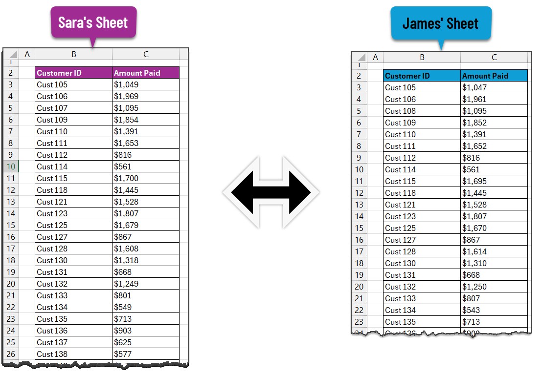
Open your Excel file and verify that your data is organized into two separate sheets. Each sheet should contain the data you want to compare. For instance, one sheet might contain data from Sara, and the other from James. Ensure both datasets have identical columns for effective matching.
2.2 Ensuring Identical Columns
Both datasets should have the same columns, though the data within them might differ. This consistency is essential for VLOOKUP to work correctly.
Alt Text: Comparing customer payment data in two Excel sheets, one with Sara’s data and another with James’ data, highlighting the need for identical columns for effective data reconciliation using VLOOKUP.
3. Initiating the VLOOKUP Formula
Begin by navigating to the first sheet. Here, you’ll use VLOOKUP (or XLOOKUP, if you’re using Excel 365) to retrieve the matching values from the second sheet.
3.1 Locating the First Sheet
Go to the first sheet in your Excel file. This is where you will input the VLOOKUP formula.
3.2 Using VLOOKUP or XLOOKUP
Depending on your Excel version, use VLOOKUP or XLOOKUP. XLOOKUP is available in Excel 365 and offers some advantages over VLOOKUP, such as better handling of missing values and more straightforward syntax.
3.3 Identifying a Unique Identifier
For this comparison, a unique identifier column such as “Customer ID” or “Invoice Number” is essential. This column will serve as the basis for matching data between the two sheets.
3.4 Setting Up the Formula
In the adjacent column, insert the VLOOKUP function to fetch corresponding values for each Customer ID from the second sheet. The initial setup should resemble this:
Alt Text: Setting up an Excel spreadsheet for comparing two sheets using VLOOKUP, emphasizing the importance of a unique identifier column like Customer ID for matching data.
4. Writing the VLOOKUP Formula
The VLOOKUP formula is the core of this comparison method. Here’s how to write and understand it.
4.1 Basic VLOOKUP Formula
Here’s an example of the VLOOKUP formula:
=VLOOKUP(B3,'James Sheet'!$B$3:$C$32,2,FALSE)4.2 Understanding the VLOOKUP Formula
- VLOOKUP: This function searches for a value in the first column of a range and returns a value from a specified column in the same row.
- B3: This is the cell containing the Customer ID you’re searching for.
- ‘James Sheet’!$B$3:$C$32: This is the range in the second sheet where the data is located. The dollar signs ($) make the reference absolute, so it doesn’t change when you drag the formula down.
- 2: This specifies that the value from the second column of the range should be returned (the “Amount Paid” column in this case).
- FALSE: This ensures that VLOOKUP looks for an exact match.
4.3 XLOOKUP as an Alternative
If you prefer using XLOOKUP, the formula would look like this:
=XLOOKUP(B3,'James Sheet'!$B$3:$B$32,'James Sheet'!$C$3:$C$32, "ID missing")4.4 Understanding the XLOOKUP Formula
- XLOOKUP: This is a more modern and flexible alternative to VLOOKUP.
- B3: The lookup value (Customer ID).
- ‘James Sheet’!$B$3:$B$32: The lookup array (range of Customer IDs in the second sheet).
- ‘James Sheet’!$C$3:$C$32: The return array (range of “Amount Paid” values in the second sheet).
- “ID missing”: This is the value returned if no match is found.
Alt Text: Illustrating the VLOOKUP formula in Excel for comparing two sheets, breaking down each component to clarify how it retrieves matching values based on Customer ID.
4.5 Applying the Formula
Apply this formula by dragging it down to fill the cells, allowing you to view matching values from the second sheet.
4.6 Handling Missing IDs
If some IDs are missing in the second sheet, the corresponding cells will display an #N/A error.
Alt Text: Displaying the #N/A error in VLOOKUP when an ID is missing in the second worksheet, indicating the need for error handling or alternative matching techniques.
5. Reconciling the Values
Once you have the matching values from the second sheet, you can reconcile the data to identify matches and discrepancies.
5.1 Using the IF Formula
Use the IF formula to compare the values in both sheets:
=IF(ISERROR(D3),"ID Missing", IF(D3<>C3,"Not matching", "Matching"))5.2 Understanding the IF Formula
- IF(ISERROR(D3),”ID Missing”, …): This checks if the VLOOKUP result is an error (#N/A), indicating a missing ID.
- IF(D3<>C3,”Not matching”, “Matching”): If there’s no error, this compares the value from the second sheet (D3) with the value from the first sheet (C3). If they are different, it flags them as “Not matching”; otherwise, it marks them as “Matching”.
5.3 Applying the Reconciliation Formula
Drag the formula down to apply it to all rows, providing reconciliation information for your data.
Alt Text: Showing the completed reconciliation of data in Excel, using IF and ISERROR functions to flag matching, non-matching, and missing IDs between two sheets.
5.4 Using Filters for Analysis
Employ Excel’s filtering capabilities to quickly view matching or non-matching records.
6. Conditional Formatting for Enhanced Visibility
To make discrepancies even more visible, use conditional formatting to highlight non-matching records.
6.1 Selecting the Data Range
Select the entire range of data you want to analyze (e.g., B3:E32).
6.2 Accessing Conditional Formatting
Go to the “Home” tab on the Excel ribbon and click on “Conditional Formatting,” then select “New Rule.”
6.3 Creating a New Rule
Choose “Use a formula to determine which cells to format.”
6.4 Entering the Formula
Type the formula =$E3="Not matching" (refer to the reconciliation column).
6.5 Setting the Format
Set the formatting to highlight the non-matching records with a specific color.
6.6 Adding a Rule for Missing IDs
Repeat the process to add another rule for “ID missing,” using the formula =$E3="ID Missing" and a different highlight color.
Alt Text: Highlighting unmatched values in Excel using conditional formatting, clearly distinguishing non-matching and missing ID records for efficient data reconciliation.
6.7 Viewing Highlighted Data
Now, all non-matching and missing ID values will be highlighted in different colors, making them easy to identify.
7. Additional Techniques for Comparing Excel Sheets
While VLOOKUP is efficient, Excel offers other methods for comparing spreadsheets.
7.1 Using MATCH Function
The MATCH function can find the position of an item in a range. You can use it to check if a value exists in another sheet.
7.2 Using INDEX and MATCH
Combining INDEX and MATCH provides a more flexible alternative to VLOOKUP, especially when dealing with complex data structures.
7.3 Using COUNTIF Function
The COUNTIF function counts the number of cells that meet a criterion. Use it to check if a value from one sheet appears in another.
7.4 Using Comparison Formulas
Simple comparison formulas (e.g., =Sheet1!A1=Sheet2!A1) can quickly highlight differences between corresponding cells.
7.5 Using Excel’s Built-in Compare Feature
Excel has a built-in feature for comparing sheets, though it may not be as flexible as VLOOKUP.
8. Practical Examples of Using VLOOKUP for Comparison
VLOOKUP can be used in various scenarios for comparing data between Excel sheets.
8.1 Comparing Customer Lists
Suppose you have two lists of customers and want to find out which customers are present in both lists. Use VLOOKUP to match Customer IDs and identify the common customers.
8.2 Comparing Inventory Records
If you have inventory records in two different sheets, VLOOKUP can help you find discrepancies in stock levels or product details.
8.3 Comparing Sales Data
For sales data across different periods, VLOOKUP can match sales records and identify changes in sales volumes or prices.
8.4 Comparing Employee Data
When managing employee information, VLOOKUP can help compare employee records between different departments or time periods to identify discrepancies.
8.5 Comparing Financial Data
In financial analysis, VLOOKUP can be used to compare financial statements, track transactions, and reconcile accounts.
9. Common Issues and Troubleshooting Tips
When using VLOOKUP to compare Excel sheets, you might encounter some common issues. Here are some troubleshooting tips.
9.1 #N/A Errors
- Issue: VLOOKUP returns #N/A when it can’t find a match.
- Solution: Ensure the lookup value exists in the lookup range. Check for typos or inconsistencies in the data.
9.2 Incorrect Results
- Issue: VLOOKUP returns a value, but it’s not the correct one.
- Solution: Double-check the column index number. Make sure you are returning the correct column.
9.3 Performance Issues
- Issue: VLOOKUP is slow when dealing with large datasets.
- Solution: Use XLOOKUP if available. Ensure your data is sorted. Consider using array formulas or other more efficient methods.
9.4 Data Type Mismatch
- Issue: VLOOKUP doesn’t find matches due to different data types (e.g., number vs. text).
- Solution: Ensure both lookup value and the lookup range have the same data type. Use functions like VALUE or TEXT to convert data types.
9.5 Case Sensitivity
- Issue: VLOOKUP is case-sensitive, and the lookup fails because of case differences.
- Solution: Use a helper column with the LOWER or UPPER function to convert both the lookup value and the lookup range to the same case.
10. Advanced VLOOKUP Techniques for Comparison
For more complex comparisons, consider these advanced VLOOKUP techniques.
10.1 Using VLOOKUP with Multiple Criteria
To compare data based on multiple criteria, create a helper column that concatenates the criteria and use this helper column as the lookup value.
10.2 Using VLOOKUP with Approximate Match
When dealing with ranges of values, use VLOOKUP with approximate match (TRUE) to find the closest match within a range.
10.3 Using VLOOKUP with Array Formulas
Array formulas can perform complex comparisons across multiple rows or columns, providing more flexible matching options.
10.4 Using VLOOKUP with Dynamic Ranges
Define dynamic ranges using functions like OFFSET or INDEX to ensure your VLOOKUP formulas automatically adjust to changes in data size.
10.5 Combining VLOOKUP with Other Functions
Combine VLOOKUP with functions like IFERROR, SUMIF, or AVERAGEIF to perform more sophisticated data analysis and reconciliation.
11. Conclusion: Simplify Data Comparison with VLOOKUP
Using VLOOKUP in Excel is a straightforward method for comparing data across two sheets, identifying matches, and highlighting discrepancies. Whether you are reconciling financial records, comparing customer lists, or managing inventory, VLOOKUP provides a powerful tool for data analysis. With the insights from COMPARE.EDU.VN, you can master VLOOKUP and similar tools to make informed decisions.
Remember, accurate data comparison is crucial for making informed decisions. For a comprehensive understanding of Excel functions and to ensure the accuracy of your comparisons, visit COMPARE.EDU.VN. Our platform offers in-depth comparisons, detailed analyses, and expert insights to help you navigate the complexities of data management.
Need more help with Excel or other comparison tasks? Contact us at:
- Address: 333 Comparison Plaza, Choice City, CA 90210, United States
- WhatsApp: +1 (626) 555-9090
- Website: compare.edu.vn
12. FAQ: Mastering VLOOKUP for Data Comparison
12.1 What is VLOOKUP and how does it work in Excel?
VLOOKUP (Vertical Lookup) is an Excel function that searches for a value in the first column of a range and returns a value from a specified column in the same row. It’s used to find matching data between different sheets or tables.
12.2 Can VLOOKUP compare data in two different Excel files?
Yes, VLOOKUP can compare data in two different Excel files. You need to specify the correct file path in the VLOOKUP formula.
12.3 What does the #N/A error mean in VLOOKUP and how can I fix it?
The #N/A error means that VLOOKUP couldn’t find a match for the lookup value in the specified range. To fix it, ensure the lookup value exists in the lookup range, check for typos, and verify that the data types match.
12.4 How do I use VLOOKUP to find differences between two Excel sheets?
Use VLOOKUP to retrieve matching values from the second sheet into the first sheet. Then, use an IF formula to compare the values and identify differences.
12.5 Is VLOOKUP case-sensitive? How can I perform a case-insensitive lookup?
Yes, VLOOKUP is case-sensitive. To perform a case-insensitive lookup, use helper columns with the LOWER or UPPER function to convert both the lookup value and the lookup range to the same case.
12.6 Can I use VLOOKUP with multiple criteria?
Yes, but it requires creating a helper column that concatenates the multiple criteria into a single lookup value. Then, use this helper column in the VLOOKUP formula.
12.7 What is XLOOKUP and how is it better than VLOOKUP?
XLOOKUP is a more modern and flexible alternative to VLOOKUP, available in Excel 365. It offers better handling of missing values, more straightforward syntax, and doesn’t require specifying a column index number.
12.8 How can I improve the performance of VLOOKUP when working with large datasets?
To improve performance, use XLOOKUP if available, ensure your data is sorted, and consider using array formulas or other more efficient methods.
12.9 Can VLOOKUP return multiple values based on a single lookup value?
No, VLOOKUP can only return one value. To return multiple values, you can use multiple VLOOKUP formulas with different column index numbers or consider using array formulas or other functions like INDEX and MATCH.
12.10 What are some common mistakes to avoid when using VLOOKUP?
Common mistakes include incorrect column index numbers, forgetting to use absolute references ($) for the lookup range, and not checking for #N/A errors. Always double-check your formula and data to avoid these mistakes.