How Do I Use Lookup in Excel to Compare Two Sheets?

Using lookup functions in Excel is an efficient way to compare two sheets. At COMPARE.EDU.VN, we understand the need for accurate data comparison. This guide will show you how to use VLOOKUP or XLOOKUP to reconcile data between two Excel sheets. Learn the steps to reconcile your data accurately, find missing information, and highlight discrepancies. This technique is vital for data validation, financial analysis, and reporting. Discover how these functions streamline data comparison and enhance decision-making in various professional settings.

1. Understanding the Need to Compare Two Excel Sheets

The ability to compare two Excel sheets efficiently is essential in various professional contexts. Whether you’re reconciling financial data, verifying inventory lists, or ensuring consistency across different versions of a report, knowing how to compare data accurately is crucial. Excel’s lookup functions, such as VLOOKUP and XLOOKUP, provide powerful tools to streamline this process. Understanding why and when to use these functions can save time, reduce errors, and improve overall data integrity.

Data Validation: Ensuring that data entered in one sheet matches the corresponding data in another.
Financial Reconciliation: Comparing financial statements from different periods or sources to identify discrepancies.
Inventory Management: Matching inventory records to track stock levels and identify shortages or overages.
Reporting Consistency: Verifying that data presented in different reports is consistent and accurate.
Version Control: Comparing different versions of a spreadsheet to track changes and ensure data integrity.

2. What are Excel Lookup Functions?

Excel lookup functions are powerful tools that allow you to find specific data within a spreadsheet based on a search criterion. These functions are particularly useful when comparing data between two sheets, as they can automatically search for matching values and return corresponding information. Two of the most commonly used lookup functions are VLOOKUP and XLOOKUP.

VLOOKUP (Vertical Lookup): Searches for a value in the first column of a range and returns a value in the same row from a specified column.
XLOOKUP: A more versatile function that can search in any column and return a value from any other column, offering improved flexibility and ease of use.

2.1. VLOOKUP Function

VLOOKUP, or Vertical Lookup, is one of Excel’s most widely used functions for searching and retrieving data. It searches for a value in the first column of a specified range and returns a corresponding value from a column you designate in the same row. VLOOKUP is particularly useful when you need to find a specific piece of information in a large dataset or compare data across multiple sheets.

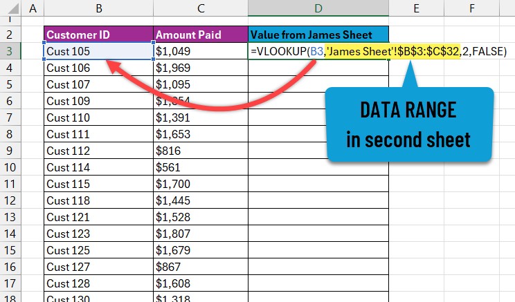
Syntax: VLOOKUP(lookup_value, table_array, col_index_num, [range_lookup])
- lookup_value: The value you want to search for.
- table_array: The range of cells where you want to search.
- col_index_num: The column number in the table_array from which to return a value.
- [range_lookup]: Optional. TRUE for approximate match (default) or FALSE for exact match.
Example: =VLOOKUP(B3,'James Sheet'!$B$3:$C$32,2,FALSE)
- Searches for the value in cell B3 within the range B3:C32 on the “James Sheet”.
- Returns the value from the second column (column C) if an exact match is found.
Limitations: VLOOKUP can only search in the first column of the specified range and may return incorrect results if the data is not properly sorted when using approximate match.

2.2. XLOOKUP Function

XLOOKUP is a modern and more flexible alternative to VLOOKUP. Introduced in Excel 365, it overcomes many of VLOOKUP’s limitations by allowing you to search in any column and return a value from any other column. XLOOKUP also offers improved error handling and default matching behavior, making it easier to use and more reliable.

Syntax: XLOOKUP(lookup_value, lookup_array, return_array, [if_not_found], [match_mode], [search_mode])
- lookup_value: The value you want to search for.
- lookup_array: The range of cells to search within.
- return_array: The range of cells from which to return a value.
- [if_not_found]: Optional. The value to return if no match is found.
- [match_mode]: Optional. Specifies the type of match (0 for exact match).
- [search_mode]: Optional. Specifies the search direction.
Example: =XLOOKUP(B3,'James Sheet'!$B$3:$B$32,'James Sheet'!$C$3:$C$32, "ID missing")
- Searches for the value in cell B3 within the range B3:B32 on the “James Sheet”.
- Returns the corresponding value from the range C3:C32.
- If no match is found, returns “ID missing”.
Advantages: XLOOKUP offers greater flexibility, improved error handling, and the ability to search in any column, making it a superior choice for many data lookup scenarios.

3. Step-by-Step Guide: How to Use Lookup in Excel to Compare Two Sheets

Comparing two Excel sheets using lookup functions involves a structured approach to ensure accuracy and efficiency. The following steps will guide you through the process using both VLOOKUP and XLOOKUP.

3.1. Setting Up Your Data in Two Excel Sheets

Before you can start comparing data, you need to organize your information in two separate sheets within the same Excel file. Ensure that both sheets have a common identifier, such as a Customer ID or Invoice Number, which will serve as the basis for your lookup.

Open Excel: Launch Microsoft Excel and create a new workbook.
Create Two Sheets: Name the first sheet “Sara’s Data” and the second sheet “James’ Data”.
Copy Data: Copy the data from your two sources into the respective sheets. Ensure that both datasets have identical columns, even if the data within those columns is not the same.
Unique Identifier: Identify a column that contains a unique identifier, such as “Customer ID” or “Invoice Number.” This column will be used to match records between the two sheets.

3.2. Using VLOOKUP to Find Matching Values

VLOOKUP can be used to search for values from one sheet in another, allowing you to compare corresponding data.

Select First Sheet: Go to the first sheet (“Sara’s Data”).
Choose Adjacent Column: In the column next to the unique identifier (e.g., Customer ID), prepare to enter the VLOOKUP formula.
Enter VLOOKUP Formula: In the first cell of the adjacent column (e.g., D3), enter the VLOOKUP formula:

=VLOOKUP(B3,'James Sheet'!$B$3:$C$32,2,FALSE)

B3: Refers to the cell with the Customer ID in the first sheet.
'James Sheet'!$B$3:$C$32: Is the range of data in the second sheet where you are trying to find a match.
2: Is the column number in the second sheet (“James’ Data”) that contains the data you want to retrieve (e.g., “Amount Paid”).
FALSE: Ensures that VLOOKUP looks for an exact match.

Fill Down the Formula: Drag the fill handle (the small square at the bottom right of the cell) down to apply the formula to all rows in your data.

3.3. Using XLOOKUP to Find Matching Values

If you have Excel 365, XLOOKUP offers a more flexible and powerful way to find matching values.

Select First Sheet: Go to the first sheet (“Sara’s Data”).
Choose Adjacent Column: In the column next to the unique identifier (e.g., Customer ID), prepare to enter the XLOOKUP formula.
Enter XLOOKUP Formula: In the first cell of the adjacent column (e.g., D3), enter the XLOOKUP formula:

=XLOOKUP(B3,'James Sheet'!$B$3:$B$32,'James Sheet'!$C$3:$C$32, "ID missing")

B3: Refers to the cell with the Customer ID in the first sheet.
'James Sheet'!$B$3:$B$32: Is the range in the second sheet where you are searching for the Customer ID.
'James Sheet'!$C$3:$C$32: Is the range in the second sheet that contains the data you want to retrieve (e.g., “Amount Paid”).
"ID missing": Is the value to return if no match is found.

Fill Down the Formula: Drag the fill handle down to apply the formula to all rows in your data.

3.4. Reconciling Values with the IF Function

Once you have retrieved the matching values from the second sheet, you can use the IF function to compare the values and identify discrepancies.

Choose Another Adjacent Column: In the next available column (e.g., E3), enter the IF formula to compare the values from the two sheets.

=IF(ISERROR(D3),"ID Missing", IF(D3<>C3,"Not matching", "Matching"))

ISERROR(D3): Checks if the VLOOKUP or XLOOKUP formula in column D returned an error (e.g., #N/A, indicating a missing ID).
"ID Missing": If there is an error, this indicates that the Customer ID is missing in the second sheet.
D3<>C3: Compares the value retrieved from the second sheet (column D) with the corresponding value in the first sheet (column C).
"Not matching": If the values are different, this indicates a discrepancy.
"Matching": If the values are the same, this indicates that the data matches.

Fill Down the Formula: Drag the fill handle down to apply the formula to all rows in your data.

3.5. Using Filters to Analyze Results

Excel’s filter feature allows you to quickly analyze the results of your comparison by isolating matching, non-matching, and missing records.

Select Data Range: Select the entire range of data, including the columns with the VLOOKUP/XLOOKUP results and the IF formula results.
Apply Filter: Go to the “Data” tab in the Excel ribbon and click on “Filter.”
Filter Options: Click on the filter dropdown in the column with the IF formula results (e.g., column E).
Select Criteria: Choose the filter criteria you want to analyze:
- “Matching”: To see only the records where the data matches in both sheets.
- “Not matching”: To see only the records where the data differs.
- “ID Missing”: To see only the records where the Customer ID is missing in the second sheet.
Analyze Results: Excel will display only the records that meet your selected criteria, allowing you to focus on specific areas of interest.

3.6. Conditional Formatting for Visual Highlighting

Conditional formatting can be used to visually highlight discrepancies and missing data, making it easier to identify and address issues.

Select Data Range: Select the range of data you want to format (e.g., B3:E32).
Open Conditional Formatting: Go to the “Home” tab in the Excel ribbon and click on “Conditional Formatting.”
New Rule: Select “New Rule…” from the dropdown menu.
Choose Rule Type: Select “Use a formula to determine which cells to format.”
Enter Formula: Enter the following formula to highlight non-matching records:

=$E3="Not matching"

$E3: Refers to the first cell in the column with the IF formula results.

Format: Click on the “Format…” button to choose the formatting style (e.g., fill color, font color) to highlight the non-matching records.
Add Rule for Missing IDs: Repeat steps 3-6 to add another rule for highlighting missing IDs:

=$E3="ID Missing"

Apply Formatting: Click “OK” to apply the conditional formatting rules. Excel will now automatically highlight the non-matching and missing ID values based on your specified formatting styles.

4. Advanced Techniques for Comparing Excel Sheets

Beyond the basic VLOOKUP and XLOOKUP methods, there are several advanced techniques that can enhance your ability to compare Excel sheets. These techniques include using array formulas, INDEX-MATCH, and specialized Excel add-ins.

4.1. Using Array Formulas

Array formulas allow you to perform complex calculations on multiple values at once. They can be particularly useful when comparing entire columns or ranges of data.

Select Output Range: Select a range of cells where you want to display the comparison results.
Enter Array Formula: Enter the array formula in the first cell of the selected range. For example, to compare two columns (A1:A10 and B1:B10) and return “Match” or “Mismatch,” you can use the following formula:

=IF(A1:A10=B1:B10, "Match", "Mismatch")

Enter as Array Formula: Press Ctrl + Shift + Enter to enter the formula as an array formula. Excel will automatically add curly braces {} around the formula.
Analyze Results: The selected range will now display “Match” or “Mismatch” for each corresponding row in the two columns.

4.2. INDEX-MATCH as an Alternative to VLOOKUP

INDEX-MATCH is a powerful alternative to VLOOKUP that offers greater flexibility and overcomes some of VLOOKUP’s limitations. It allows you to search for values in any column and return corresponding values from any other column.

Select Output Cell: Select the cell where you want to display the result.
Enter INDEX-MATCH Formula: Enter the INDEX-MATCH formula. For example:

=INDEX('James Sheet'!$C$3:$C$32, MATCH(B3, 'James Sheet'!$B$3:$B$32, 0))

'James Sheet'!$C$3:$C$32: Is the range containing the values you want to return.
MATCH(B3, 'James Sheet'!$B$3:$B$32, 0): Finds the row number where the value in B3 (from “Sara’s Data”) matches in the range B3:B32 (in “James’ Data”).
0: Specifies an exact match.

Fill Down the Formula: Drag the fill handle down to apply the formula to all rows in your data.

4.3. Using Excel Add-ins for Advanced Comparison

Several Excel add-ins are specifically designed for advanced data comparison and reconciliation. These add-ins offer features such as detailed change tracking, side-by-side comparison views, and automated reconciliation processes.

Spreadsheet Compare: A built-in Excel tool (available in some versions) that allows you to compare two workbooks and highlight differences.
Beyond Compare: A third-party tool that offers advanced file comparison features, including the ability to compare Excel files.
XL Comparator: An Excel add-in that provides detailed comparison reports and change tracking.

5. Practical Examples of Using Lookup Functions for Data Comparison

To illustrate the practical applications of using lookup functions for data comparison, let’s consider a few real-world scenarios.

5.1. Example 1: Reconciling Financial Data

Imagine you are an accountant tasked with reconciling two sets of financial data: one from your accounting software and another from a third-party payment processor.

Data Setup: Copy the data from both sources into separate sheets in an Excel file.
Unique Identifier: Use a unique transaction ID to match records between the two sheets.
VLOOKUP/XLOOKUP: Use VLOOKUP or XLOOKUP to retrieve the corresponding transaction amounts from the payment processor’s data into the accounting software’s sheet.
IF Function: Use the IF function to compare the transaction amounts and flag any discrepancies.
Conditional Formatting: Use conditional formatting to highlight the discrepancies for further investigation.

5.2. Example 2: Verifying Inventory Lists

Suppose you are a warehouse manager responsible for verifying inventory lists from two different warehouses.

Data Setup: Copy the inventory lists into separate sheets in an Excel file.
Unique Identifier: Use a unique product SKU to match records between the two sheets.
VLOOKUP/XLOOKUP: Use VLOOKUP or XLOOKUP to retrieve the quantity of each product from the second warehouse’s list into the first warehouse’s sheet.
IF Function: Use the IF function to compare the quantities and identify any discrepancies.
Filters: Use filters to analyze the results and identify products with significant quantity differences.

5.3. Example 3: Tracking Sales Performance

Consider a sales manager who wants to compare the sales performance of two different sales teams.

Data Setup: Copy the sales data for each team into separate sheets in an Excel file.
Unique Identifier: Use a unique sales representative ID to match records between the two sheets.
VLOOKUP/XLOOKUP: Use VLOOKUP or XLOOKUP to retrieve the sales revenue for each representative from the second team’s data into the first team’s sheet.
IF Function: Use the IF function to compare the sales revenue and identify any performance differences.
Charts: Create charts to visualize the sales performance differences between the two teams.

6. Common Issues and Troubleshooting Tips

While using lookup functions in Excel can be highly efficient, you may encounter some common issues. Here are some troubleshooting tips to help you resolve these problems:

#N/A Error: This error indicates that the lookup value was not found in the specified range.
- Check Lookup Value: Ensure that the lookup value exists in the second sheet.
- Verify Range: Make sure that the specified range is correct and includes the lookup column.
- Exact Match: Ensure that the range_lookup argument in VLOOKUP is set to FALSE for an exact match.
Incorrect Results: If the lookup function returns incorrect results, it may be due to the following reasons:
- Incorrect Column Index: Verify that the col_index_num argument in VLOOKUP is correct and points to the correct column.
- Data Type Mismatch: Ensure that the data types of the lookup value and the values in the lookup column are the same.
- Sorting Issues: If using approximate match (TRUE in VLOOKUP), ensure that the lookup column is sorted in ascending order.
Performance Issues: When working with large datasets, lookup functions can slow down Excel’s performance.
- Optimize Formulas: Use named ranges instead of cell references to improve formula readability and performance.
- Reduce Volatile Functions: Avoid using volatile functions like NOW() and TODAY() in your lookup formulas.
- Use Excel Tables: Convert your data ranges into Excel tables to improve performance.

7. The Benefits of Using COMPARE.EDU.VN for Data Comparison

COMPARE.EDU.VN offers comprehensive resources and tools to simplify the process of data comparison and decision-making. Our platform provides detailed comparisons, expert reviews, and user feedback to help you make informed choices.

7.1. Access to Detailed Comparisons

COMPARE.EDU.VN provides detailed comparisons across a wide range of products, services, and ideas. Our comparisons are meticulously researched and presented in an easy-to-understand format, allowing you to quickly identify the key differences and make informed decisions.

7.2. Expert Reviews and User Feedback

Our platform features expert reviews and user feedback to provide you with a well-rounded perspective on the options you are considering. Benefit from the insights of industry professionals and the experiences of other users to gain a deeper understanding of the strengths and weaknesses of each choice.

7.3. Tools and Resources for Decision-Making

COMPARE.EDU.VN offers a variety of tools and resources to assist you in the decision-making process. From interactive comparison tables to customizable checklists, we provide the tools you need to evaluate your options and select the best fit for your needs.

8. Why Choose COMPARE.EDU.VN?

At COMPARE.EDU.VN, we are committed to providing you with the most accurate and comprehensive information possible. Our team of experts works tirelessly to research and analyze data from multiple sources, ensuring that our comparisons are unbiased and reliable.

8.1. Accuracy and Reliability

We prioritize accuracy and reliability in all of our comparisons. Our team of experts conducts thorough research and analysis to ensure that the information we provide is up-to-date and trustworthy.

8.2. Comprehensive Information

COMPARE.EDU.VN offers comprehensive information on a wide range of topics. Whether you are comparing products, services, or ideas, you can rely on us to provide you with the details you need to make informed decisions.

8.3. User-Friendly Interface

Our platform is designed to be user-friendly and intuitive. Easily navigate through our comparisons and access the information you need without any hassle.

9. Conclusion: Streamline Data Comparison with Excel and COMPARE.EDU.VN

Using lookup functions in Excel, such as VLOOKUP and XLOOKUP, is a powerful way to compare data between two sheets. These functions allow you to quickly find matching values, identify discrepancies, and reconcile data efficiently. By following the step-by-step guide outlined in this article, you can streamline your data comparison tasks and improve your overall data management practices.

For more comprehensive comparisons and expert insights, visit COMPARE.EDU.VN. Our platform offers a wealth of resources to help you make informed decisions and optimize your data analysis processes.

Contact us today at 333 Comparison Plaza, Choice City, CA 90210, United States, or reach out via WhatsApp at +1 (626) 555-9090. Visit our website at compare.edu.vn to explore our extensive comparison tools and resources.

10. Frequently Asked Questions (FAQs)

10.1. Can I use VLOOKUP to compare more than two sheets?

Yes, you can use VLOOKUP to compare more than two sheets by nesting multiple VLOOKUP functions or combining VLOOKUP with other functions like IF and ISERROR. However, for comparing multiple sheets, consider using Power Query, which is more efficient for complex comparisons.

10.2. What is the main difference between VLOOKUP and XLOOKUP?

The main differences between VLOOKUP and XLOOKUP are flexibility and ease of use. XLOOKUP can search in any column and return values from any other column, while VLOOKUP is limited to searching in the first column of the range. XLOOKUP also offers better default matching and error handling.

10.3. How do I handle errors when using VLOOKUP or XLOOKUP?

To handle errors, you can use the IFERROR function in combination with VLOOKUP or XLOOKUP. For example:
=IFERROR(VLOOKUP(A2,Sheet2!A:B,2,FALSE), "Not Found")
This formula will return “Not Found” if VLOOKUP returns an error.

10.4. Can I compare data in two Excel files instead of two sheets?

Yes, you can compare data in two Excel files by referencing the external file in your VLOOKUP or XLOOKUP formula. For example:
=VLOOKUP(A2,'[FileName.xlsx]Sheet1'!$A:$B,2,FALSE)
Make sure the external file is open, or provide the full path to the file.

10.5. How do I compare two columns for exact matches and highlight the differences?

You can compare two columns for exact matches using the IF function and conditional formatting. For example:
=IF(A2=B2, "Match", "Mismatch")
Then, use conditional formatting to highlight the “Mismatch” cells.

10.6. What is the best way to compare large datasets in Excel?

For large datasets, using Power Query (Get & Transform Data) is more efficient than VLOOKUP or XLOOKUP. Power Query can handle large amounts of data and perform complex comparisons and transformations.

10.7. How can I find the differences between two lists in Excel?

You can find the differences between two lists using a combination of VLOOKUP and ISNA. For example:
=IF(ISNA(VLOOKUP(A2,List2!A:A,1,FALSE)), "Unique to List1", "")
This formula will identify items in List1 that are not in List2.

10.8. Can I use wildcards in VLOOKUP or XLOOKUP to find partial matches?

Yes, you can use wildcards in VLOOKUP and XLOOKUP for partial matches. For example:
=VLOOKUP("*"&A2&"*",Sheet2!A:B,2,FALSE)
This will find the first value that contains the value in A2.

10.9. How do I compare data based on multiple criteria?

You can compare data based on multiple criteria by creating a helper column that concatenates the criteria and then using VLOOKUP or XLOOKUP on the helper column.

10.10. Is there a way to automate the comparison process in Excel?

Yes, you can automate the comparison process in Excel using VBA (Visual Basic for Applications). VBA allows you to write custom code to perform complex comparisons and generate reports automatically.