How To Use Conditional Formatting To Compare Two Cells?

Using conditional formatting to compare two cells in Excel allows you to visually highlight differences or similarities, aiding in data analysis and decision-making, all available on COMPARE.EDU.VN. This guide explores how to leverage this feature effectively. Understanding this technique will enable you to pinpoint discrepancies and trends, turning raw data into actionable insights.

1. What is Conditional Formatting and Why Compare Cells?

Conditional formatting is a feature in Excel that allows you to automatically apply formatting to cells based on certain criteria. Comparing cells using conditional formatting enables you to quickly identify differences, similarities, or patterns between data entries, enhancing data analysis and decision-making.

1.1. Understanding Conditional Formatting

Conditional formatting in Excel is a powerful tool that lets you automatically format cells based on specific criteria. This formatting can include changes to cell color, font, borders, and even the addition of icons or data bars. The primary purpose of conditional formatting is to visually highlight important information, trends, or anomalies in your data, making it easier to analyze and interpret.

For instance, you can set up a rule to highlight all sales figures above a certain target in green, or flag values below a threshold in red. This immediate visual feedback helps you quickly identify key data points without manually sifting through rows and columns. The flexibility of conditional formatting extends to various scenarios, from tracking project timelines to monitoring inventory levels, making it an indispensable tool for data-driven decision-making.

1.2. Why Compare Cells?

Comparing cells is crucial for data validation, identifying trends, and making informed decisions. By visually highlighting the differences or similarities between cells, you can quickly identify errors, outliers, or patterns that might otherwise go unnoticed.

Comparing cells enables users to pinpoint discrepancies, validate data entry, and ensure data integrity. Identifying trends and patterns becomes more manageable when data is visually represented, allowing for quicker analysis and more informed decision-making.

For example, a sales manager can compare current sales figures against previous periods to identify growth trends or potential downturns. An accountant can compare expenses against budget to highlight areas where cost-cutting measures may be needed. In each of these scenarios, the ability to quickly and easily compare cells using conditional formatting can save time and improve accuracy.

1.3. Benefits of Using Conditional Formatting for Cell Comparison

Using conditional formatting to compare cells offers several advantages:

Time-saving: Quickly identify differences without manual inspection.
Improved accuracy: Reduce the risk of overlooking important discrepancies.
Enhanced data visualization: Gain insights through visually highlighted data.
Better decision-making: Make informed decisions based on clear data patterns.

Conditional formatting allows for real-time updates, meaning that as data changes, the formatting automatically adjusts to reflect those changes. This dynamic capability ensures that insights remain current and relevant. By making data analysis faster, more accurate, and more visually engaging, conditional formatting becomes an indispensable tool for anyone working with spreadsheets.

2. Key Concepts for Conditional Formatting in Excel

Before diving into specific examples, understanding key concepts like absolute and relative references, formulas, and the order of operations is essential.

2.1. Absolute and Relative Cell References

In Excel, cell references can be either relative or absolute, and understanding the difference is crucial for effective conditional formatting.

Relative References: Relative references change when a formula is copied to another cell. For example, if cell C1 contains the formula =A1+B1, and you copy this formula to cell C2, it will automatically adjust to =A2+B2. This is useful when you want the formula to adapt to the new row or column.
Absolute References: Absolute references, on the other hand, do not change when copied. To create an absolute reference, you use the $ sign before the column and/or row. For example, =$A$1 is an absolute reference to cell A1, and it will always refer to that cell, no matter where you copy the formula. A$1 makes the row absolute while the column is relative. $A1 makes the column absolute while the row is relative.

Understanding when to use relative or absolute references is crucial for conditional formatting formulas. Typically, in conditional formatting, you want to use a combination of both. For example, if you are comparing each row to a fixed value in cell A1, you would use $A$1 to ensure that all rows are compared to that specific cell. If you want to compare each cell in a column to the corresponding cell in another column, you would use relative references like A1 and B1, so that Excel automatically adjusts the comparison for each row.

2.2. Using Formulas in Conditional Formatting

Formulas are the heart of conditional formatting, allowing you to define complex rules for when and how cells should be formatted.

Basic Formulas: Simple formulas can compare values directly, like =A1>B1 to check if the value in cell A1 is greater than the value in cell B1.
Complex Formulas: More complex formulas can use functions like AND, OR, IF, and COUNTIF to evaluate multiple conditions. For example, =AND(A1>10, B1<20) checks if the value in A1 is greater than 10 and the value in B1 is less than 20.

To use a formula in conditional formatting, you select the cells you want to format, go to Home > Conditional Formatting > New Rule, choose “Use a formula to determine which cells to format,” and then enter your formula. The formula should return TRUE for cells that you want to format and FALSE for cells that should remain unchanged. For example, if you want to highlight cells in column A that are greater than their corresponding cells in column B, you would select column A, create a new rule, and enter the formula =A1>B1.

2.3. Order of Operations and Correct Syntax

Like all formulas in Excel, conditional formatting formulas follow a specific order of operations, typically remembered by the acronym PEMDAS (Parentheses, Exponents, Multiplication and Division, Addition and Subtraction). Understanding this order is crucial to ensure your formulas are evaluated correctly.

Parentheses: Operations inside parentheses are performed first.
Exponents: Exponentiation is performed next.
Multiplication and Division: These are performed from left to right.
Addition and Subtraction: These are performed from left to right.

Correct syntax is also critical to avoid errors. Make sure to use the correct operators (=, >, <, >=, <=, <>), and enclose text strings in double quotes ("text"). When using functions, ensure that you provide the correct arguments in the right order.

For example, if you want to highlight cells where the value in column A is both greater than 10 and less than the value in column B, the correct formula would be =AND(A1>10, A1<B1). Failing to use the correct syntax or misunderstanding the order of operations can lead to unexpected results and incorrect formatting. Always double-check your formulas and test them thoroughly to ensure they work as intended.

3. Step-by-Step Guide: Comparing Two Cells with Conditional Formatting

Here’s how to set up conditional formatting to compare two cells, along with practical examples and troubleshooting tips.

3.1. Basic Comparison: Highlighting Differences

To highlight cells that are different from another cell, follow these steps:

Select the Range: Choose the range of cells you want to format.
Open Conditional Formatting: Go to Home > Conditional Formatting > New Rule.
Choose Formula Option: Select “Use a formula to determine which cells to format”.
Enter the Formula:
- To highlight cells in column A that are different from column B, enter the formula: =A1<>B1.
Set the Format: Click on “Format”, choose your desired formatting (e.g., fill color), and click “OK”.
Apply the Rule: Click “OK” in the New Formatting Rule window to apply the rule.

This method is useful for identifying discrepancies between two sets of data, such as comparing actual sales figures against projected figures.

3.2. Highlighting Based on Conditions: Greater Than or Less Than

To highlight cells based on whether they are greater than or less than another cell:

Select the Range: Choose the cells you want to format.
Open Conditional Formatting: Go to Home > Conditional Formatting > New Rule.
Choose Formula Option: Select “Use a formula to determine which cells to format”.
Enter the Formula:
- To highlight cells in column A that are greater than column B, use: =A1>B1.
- To highlight cells in column A that are less than column B, use: =A1<B1.
Set the Format: Click on “Format”, choose your desired formatting, and click “OK”.
Apply the Rule: Click “OK” in the New Formatting Rule window.

For example, a project manager can use this technique to quickly highlight tasks that are running behind schedule by comparing planned start dates against actual start dates.

3.3. Using AND/OR Functions for Complex Conditions

The AND and OR functions allow you to create more complex conditional formatting rules that depend on multiple conditions.

Select the Range: Choose the cells you want to format.
Open Conditional Formatting: Go to Home > Conditional Formatting > New Rule.
Choose Formula Option: Select “Use a formula to determine which cells to format”.
Enter the Formula:
- To highlight cells where the value in column A is greater than 10 AND less than column B, use: =AND(A1>10, A1<B1).
- To highlight cells where the value in column A is either greater than 10 OR greater than column B, use: =OR(A1>10, A1>B1).
Set the Format: Click on “Format”, choose your desired formatting, and click “OK”.
Apply the Rule: Click “OK” in the New Formatting Rule window.

For instance, a human resources manager can use this method to identify employees who meet certain performance criteria, such as having a sales record above a specific target AND a customer satisfaction rating above a certain threshold.

3.4. Formatting Entire Rows Based on One Cell’s Value

To format entire rows based on the value of a single cell:

Select the Range: Select the entire range of rows you want to format.
Open Conditional Formatting: Go to Home > Conditional Formatting > New Rule.
Choose Formula Option: Select “Use a formula to determine which cells to format”.
Enter the Formula:
- To format the entire row if the value in column A is greater than 10, use: =$A1>10. Note the use of the absolute column reference ($A).
Set the Format: Click on “Format”, choose your desired formatting, and click “OK”.
Apply the Rule: Click “OK” in the New Formatting Rule window.

A common application is in project management, where you can highlight entire rows for tasks that are marked as overdue by referencing a status column.

3.5. Practical Examples and Use Cases

Inventory Management: Highlight products where the stock level is below the reorder point.
Sales Tracking: Identify salespersons who have exceeded their monthly targets.
Project Management: Highlight tasks that are overdue or at risk of being delayed.
Budgeting: Identify expenses that exceed the budgeted amount.

These real-world examples demonstrate the versatility and practical benefits of using conditional formatting to compare cells.

3.6. Troubleshooting Common Issues

Incorrect Formatting: Ensure that the formatting options you selected are appropriate for the type of data you are comparing.
Formula Errors: Double-check your formulas for syntax errors, incorrect cell references, and logical mistakes.
Rule Conflicts: If multiple rules are applied, they may conflict with each other. Use the “Manage Rules” option to adjust the order and settings of the rules.
Range Issues: Verify that the correct range of cells is selected for the conditional formatting rule.

4. Advanced Techniques for Conditional Formatting

Take your conditional formatting skills to the next level with these advanced techniques.

4.1. Using Functions Like MATCH and INDEX

The MATCH and INDEX functions can be used to perform more complex lookups and comparisons.

MATCH: Returns the position of a specified value in a range.
INDEX: Returns the value at a given position in a range.

For example, you can use these functions to compare data in two different sheets or to find values that meet specific criteria.

4.2. Conditional Formatting Across Multiple Sheets

Conditional formatting can be applied across multiple sheets by referencing cells in other sheets within your formulas. For example, you can compare sales data from one sheet to budget data in another sheet to highlight variances.

4.3. Dynamic Conditional Formatting with Named Ranges

Named ranges allow you to create dynamic conditional formatting rules that automatically adjust as your data changes. By defining a named range, you can ensure that your conditional formatting rules always apply to the correct set of cells.

4.4. Combining Conditional Formatting with Data Validation

Combining conditional formatting with data validation can help you ensure data integrity and consistency. Data validation allows you to restrict the type of data that can be entered into a cell, while conditional formatting can highlight cells that do not meet the specified criteria.

4.5. Custom Formulas for Specific Scenarios

For highly specific scenarios, you can create custom formulas that combine multiple functions and conditions. For example, you can create a formula that highlights cells based on a combination of date, value, and status criteria.

5. Best Practices for Effective Conditional Formatting

Follow these best practices to ensure your conditional formatting is effective and efficient.

5.1. Keep It Simple and Clear

Use clear and concise formatting options that are easy to understand. Avoid using too many colors or complex patterns that can make your data difficult to interpret.

5.2. Use Consistent Formatting

Apply consistent formatting rules across your spreadsheets to ensure uniformity and clarity. This makes it easier for users to understand and interpret the data.

5.3. Document Your Rules

Keep a record of your conditional formatting rules, including the formulas used and the formatting applied. This makes it easier to maintain and update your rules over time.

5.4. Test Your Rules Thoroughly

Always test your conditional formatting rules thoroughly to ensure they work as expected. Use a variety of test cases to verify that your rules are accurate and reliable.

5.5. Optimize for Performance

Conditional formatting can impact Excel’s performance, especially with large datasets. Use conditional formatting sparingly and optimize your formulas to minimize the impact on performance.

6. How COMPARE.EDU.VN Can Help You Compare and Decide

COMPARE.EDU.VN offers a comprehensive platform for comparing various options across education, products, and services. Our detailed comparisons and user reviews help you make informed decisions.

6.1. Comprehensive Comparisons of Products and Services

COMPARE.EDU.VN provides in-depth comparisons of various products and services, including features, specifications, prices, and user reviews. Our comparisons are designed to help you quickly identify the best options for your needs.

6.2. Educational Resources for Informed Decisions

We offer a wide range of educational resources, including articles, guides, and tutorials, to help you understand the factors to consider when making a decision. Our resources cover a variety of topics, from choosing the right school to selecting the best software.

6.3. User Reviews and Ratings for Real-World Insights

COMPARE.EDU.VN features user reviews and ratings for many of the products and services we compare. These reviews provide valuable real-world insights that can help you make a more informed decision.

6.4. Tools and Templates to Simplify Your Analysis

We offer a variety of tools and templates to help you simplify your analysis and make better decisions. These tools include comparison charts, decision matrices, and other resources designed to streamline the decision-making process.

7. Conclusion

Conditional formatting is a powerful tool for comparing cells in Excel, allowing you to visually highlight differences, similarities, and patterns. By understanding the key concepts and following the step-by-step guides, you can effectively use conditional formatting to enhance your data analysis and decision-making. For more comprehensive comparisons and resources, visit COMPARE.EDU.VN.

Ready to make more informed decisions? Visit COMPARE.EDU.VN today to explore our detailed comparisons and educational resources. Whether you’re comparing products, services, or educational opportunities, we’re here to help you make the right choice.
Our services are available worldwide. Contact us at 333 Comparison Plaza, Choice City, CA 90210, United States. For immediate assistance, reach out via Whatsapp: +1 (626) 555-9090, or visit our website: compare.edu.vn

8. Frequently Asked Questions (FAQ)

8.1. Can I use conditional formatting to compare data in different sheets?

Yes, you can use conditional formatting to compare data in different sheets by referencing cells in other sheets within your formulas. For example, you can use the formula =Sheet1!A1>Sheet2!A1 to compare the value in cell A1 of Sheet1 with the value in cell A1 of Sheet2.

8.2. How do I apply conditional formatting to an entire column?

To apply conditional formatting to an entire column, select the entire column by clicking on the column header (e.g., “A” for column A). Then, create your conditional formatting rule as described in the step-by-step guide.

8.3. What should I do if my conditional formatting rule is not working?

If your conditional formatting rule is not working, double-check your formula for syntax errors, incorrect cell references, and logical mistakes. Also, verify that the correct range of cells is selected for the rule and that there are no conflicting rules.

8.4. Can I use conditional formatting to highlight duplicate values?

Yes, you can use conditional formatting to highlight duplicate values. Select the range of cells you want to check for duplicates, go to Home > Conditional Formatting > Highlight Cells Rules > Duplicate Values, and choose your desired formatting.

8.5. How do I remove conditional formatting from a cell or range of cells?

To remove conditional formatting, select the cells from which you want to remove the formatting, go to Home > Conditional Formatting > Clear Rules, and choose whether to clear rules from the selected cells or from the entire sheet.

8.6. Is it possible to use conditional formatting with text values?

Yes, conditional formatting can be used with text values. You can use formulas to compare text values, check if a cell contains a specific text string, or highlight cells that match a specific pattern.

8.7. How can I format dates using conditional formatting?

You can format dates using conditional formatting by using formulas that compare dates, check if a date is before or after a specific date, or highlight dates that fall within a specific range.

8.8. Can I copy conditional formatting rules from one cell to another?

Yes, you can copy conditional formatting rules from one cell to another using the Format Painter tool. Select the cell with the formatting you want to copy, click on the Format Painter icon (located in the Home tab), and then click on the cell or range of cells to which you want to apply the formatting.

8.9. How do I manage multiple conditional formatting rules?

To manage multiple conditional formatting rules, go to Home > Conditional Formatting > Manage Rules. In the Conditional Formatting Rules Manager window, you can view, edit, delete, and reorder your rules.

8.10. What is the impact of conditional formatting on Excel’s performance?

Conditional formatting can impact Excel’s performance, especially with large datasets. To minimize the impact on performance, use conditional formatting sparingly, optimize your formulas, and avoid using complex patterns or too many colors.

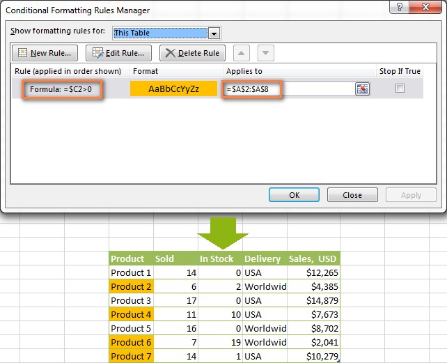Excel conditional formatting rule to highlight cells based on another cell