How To Use A Pivot Table To Compare Data?

Dive into the world of data comparison with pivot tables, a powerful tool for analyzing and summarizing information, especially with the assistance of COMPARE.EDU.VN. This guide will show you how to use pivot tables effectively, offering insights into data summarization techniques and value display options for insightful data analysis. Explore data analysis, data summarization, and reporting tools through the lens of pivot table functionality.

1. What Is A Pivot Table And Why Use It For Data Comparison?

A pivot table is a data summarization tool found in data visualization programs such as Microsoft Excel or Google Sheets. It helps organize and rearrange data in a spreadsheet to extract meaningful information. Pivot tables are particularly useful for data comparison because they allow you to quickly summarize and analyze large datasets, identify trends, and uncover relationships between different variables.

Pivot tables are useful because:

Summarization: Pivot tables can automatically sum, count, average, or perform other calculations on your data, making it easier to see the big picture.
Flexibility: You can easily rearrange the rows, columns, and values in a pivot table to explore your data from different angles.
Filtering: Pivot tables allow you to filter your data to focus on specific subsets, making it easier to compare different groups or categories.
Drill-down: You can drill down into the details of a pivot table to see the underlying data that makes up each summary value.
Visualization: Pivot tables can be used to create charts and graphs that visually represent your data, making it easier to communicate your findings to others.

2. What Are The Key Components Of A Pivot Table?

Understanding the key components of a pivot table is essential for effective data comparison. These components include:

Rows: The row labels in a pivot table are the categories or groups you want to compare. For example, if you are comparing sales data by region, the row labels might be the different regions.
Columns: The column labels in a pivot table are the variables you want to analyze. For example, if you are comparing sales data by product, the column labels might be the different products.
Values: The values in a pivot table are the summary calculations you want to perform on your data. For example, you might want to sum the sales for each region and product combination.
Filters: The filters in a pivot table allow you to focus on specific subsets of your data. For example, you might want to filter your data to only show sales for a particular year or product category.

3. How Do I Prepare My Data For Use In A Pivot Table?

Before you can use a pivot table to compare data, you need to make sure your data is properly formatted. Here are some tips for preparing your data:

Clean Your Data: Remove any errors, inconsistencies, or missing values from your data.
Organize Your Data: Arrange your data in a tabular format with clear column headers.
Use Consistent Data Types: Make sure each column contains only one type of data (e.g., numbers, text, dates).
Avoid Empty Rows and Columns: Remove any empty rows or columns from your data.
Create a Table: In Excel, format your data as a table by selecting your data and pressing Ctrl+T. This will make it easier to create and update your pivot table.

4. What Are The Steps To Create A Pivot Table In Excel?

Here are the basic steps to create a pivot table in Excel:

Select Your Data: Select the range of cells that contains the data you want to analyze.
Insert a Pivot Table: Go to the “Insert” tab on the Excel ribbon and click “PivotTable.”
Choose a Location: In the “Create PivotTable” dialog box, choose where you want to place the pivot table (e.g., a new worksheet or an existing worksheet).
Drag and Drop Fields: In the “PivotTable Fields” pane, drag and drop the fields you want to use as rows, columns, values, and filters.
Customize Your Pivot Table: Use the pivot table tools to customize the appearance and layout of your pivot table.

5. How Do I Add Fields To Rows, Columns, And Values In A Pivot Table?

Adding fields to the rows, columns, and values areas of a pivot table is the key to summarizing and comparing your data. Here’s how to do it:

Rows: Drag a field from the “PivotTable Fields” pane to the “Rows” area to create row labels in your pivot table. For example, you might drag the “Region” field to the “Rows” area to compare data by region.
Columns: Drag a field from the “PivotTable Fields” pane to the “Columns” area to create column labels in your pivot table. For example, you might drag the “Product” field to the “Columns” area to compare data by product.
Values: Drag a field from the “PivotTable Fields” pane to the “Values” area to calculate summary values in your pivot table. By default, Excel will sum the values in the field, but you can change the calculation to count, average, or other functions.

6. How Can I Change The Summary Calculation In A Pivot Table (Sum, Average, Count, Etc.)?

By default, pivot table fields placed in the Values area are displayed as a SUM. If Excel interprets your data as text, the data is displayed as a COUNT. This is why it’s so important to make sure you don’t mix data types for value fields. You can change the default calculation by first selecting the arrow to the right of the field name, and then select the Value Field Settings option.

Here’s how to change the summary calculation:

Right-Click on the Value Field: Right-click on the value field in the “Values” area of the pivot table.
Select “Value Field Settings”: In the context menu, select “Value Field Settings.”
Choose a Calculation: In the “Value Field Settings” dialog box, go to the “Summarize Values By” tab and choose the calculation you want to use (e.g., “Sum,” “Count,” “Average,” “Max,” “Min,” etc.).
Format Your Numbers: Select Number Format, you can change the number format for the entire field.
Click “OK”: Click “OK” to apply the new calculation to your pivot table.

7. How Do I Filter Data In A Pivot Table To Focus On Specific Comparisons?

Filtering data in a pivot table is a powerful way to focus on specific comparisons. Here’s how to do it:

Add a Filter Field: Drag a field from the “PivotTable Fields” pane to the “Filters” area of the pivot table.
Open the Filter Menu: Click on the filter dropdown arrow in the pivot table.
Select Filter Criteria: In the filter menu, choose the criteria you want to use to filter your data. You can select individual items or use more advanced filtering options like “Equals,” “Does Not Equal,” “Begins With,” etc.
Click “OK”: Click “OK” to apply the filter to your pivot table.

8. What Are Some Advanced Pivot Table Features For Data Comparison?

Pivot tables offer a range of advanced features that can help you compare data more effectively:

Calculated Fields: You can create calculated fields in a pivot table to perform custom calculations on your data. For example, you might create a calculated field to calculate the profit margin for each product.
Grouping: You can group items in a pivot table to create broader categories. For example, you might group individual products into product categories.
Slicers: Slicers are visual filters that make it easy to filter your data by clicking on buttons.
Timelines: Timelines are visual filters that make it easy to filter your data by date.
Pivot Charts: Pivot charts are charts that are automatically created from your pivot table data. They make it easy to visualize your data and identify trends.

9. How Can I Display Values As Percentages In A Pivot Table?

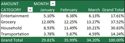
Instead of using a calculation to summarize the data, you can also display it as a percentage of a field. In the following example, we changed our household expense amounts to display as a % of Grand Total instead of the sum of the values.

Here’s how to display values as percentages:

Right-Click on the Value Field: Right-click on the value field in the “Values” area of the pivot table.
Select “Show Values As”: In the context menu, select “Show Values As.”
Choose a Percentage Option: In the “Show Values As” submenu, choose the percentage option you want to use (e.g., “% of Grand Total,” “% of Column Total,” “% of Row Total,” etc.).
Click “OK”: Click “OK” to apply the percentage calculation to your pivot table.

10. How To Display A Value As Both A Calculation And Percentage?

To display a value as both a calculation and percentage, simply drag the item into the Values section twice, and then set the Summarize Values By and Show Values As options for each one.

11. How Do I Use Slicers To Dynamically Filter Data In A Pivot Table?

Slicers provide a dynamic and visual way to filter data in a pivot table. Here’s how to use them:

Select the Pivot Table: Click on the pivot table to select it.
Insert a Slicer: Go to the “Insert” tab on the Excel ribbon and click “Slicer.”
Choose a Field: In the “Insert Slicers” dialog box, choose the field you want to use as a slicer and click “OK.”
Use the Slicer: Click on the buttons in the slicer to filter your data. You can select multiple buttons by holding down the Ctrl key.

12. Can I Create Pivot Charts Directly From My Pivot Table Data?

Yes, you can create pivot charts directly from your pivot table data. Here’s how:

Select the Pivot Table: Click on the pivot table to select it.
Insert a Pivot Chart: Go to the “Insert” tab on the Excel ribbon and click “PivotChart.”
Choose a Chart Type: In the “Insert Chart” dialog box, choose the chart type you want to use and click “OK.”

The pivot chart will automatically update as you change the layout and filters in your pivot table.

13. How Do I Group Dates Or Numbers In A Pivot Table For Better Comparison?

Grouping dates or numbers in a pivot table can help you compare data over time or across different ranges. Here’s how to do it:

Right-Click on the Field: Right-click on the date or number field in the “Rows” or “Columns” area of the pivot table.
Select “Group”: In the context menu, select “Group.”
Choose Grouping Options: In the “Grouping” dialog box, choose the grouping options you want to use (e.g., “Days,” “Months,” “Years,” or “Custom”).
Click “OK”: Click “OK” to apply the grouping to your pivot table.

14. What Is The Difference Between “Getpivotdata” And Regular Cell Referencing?

“GETPIVOTDATA” is a function in Excel that allows you to extract data from a pivot table based on specific criteria. Unlike regular cell referencing, which simply retrieves the value from a specific cell, “GETPIVOTDATA” dynamically retrieves data based on the pivot table’s structure and filters.

Here’s a comparison:

Regular Cell Referencing:
- Retrieves the value from a specific cell.
- Does not automatically update if the pivot table’s structure or filters change.
GETPIVOTDATA:
- Retrieves data from the pivot table based on specific criteria (e.g., row label, column label, filter).
- Automatically updates if the pivot table’s structure or filters change.

15. How Can Calculated Fields Enhance Data Comparison Within Pivot Tables?

Calculated fields enhance data comparison within pivot tables by allowing you to create custom calculations based on the existing data. For example, you can create a calculated field to calculate the profit margin for each product, or to calculate the percentage change in sales from one year to the next.

Here’s how to create a calculated field:

Select the Pivot Table: Click on the pivot table to select it.
Go to the “Formulas” Tab: Go to the “Formulas” tab on the Excel ribbon and click “Calculated Field.”
Enter a Name and Formula: In the “Insert Calculated Field” dialog box, enter a name for your calculated field and enter the formula you want to use.
Click “Add”: Click “Add” to add the calculated field to your pivot table.
Click “OK”: Click “OK” to close the dialog box.

16. What Are Some Common Mistakes To Avoid When Using Pivot Tables?

Here are some common mistakes to avoid when using pivot tables:

Using Unclean Data: Make sure your data is clean and consistent before creating a pivot table.
Mixing Data Types: Avoid mixing data types in the same column (e.g., numbers and text).
Forgetting to Refresh: Refresh your pivot table after making changes to your data.
Overcomplicating the Layout: Keep your pivot table layout simple and easy to understand.
Ignoring the Underlying Data: Remember to drill down into the details of your pivot table to understand the underlying data.

17. How Do I Update A Pivot Table When The Source Data Changes?

To update a pivot table when the source data changes, simply refresh the pivot table. Here’s how:

Select the Pivot Table: Click on the pivot table to select it.
Refresh the Pivot Table: Go to the “Data” tab on the Excel ribbon and click “Refresh.”

You can also set the pivot table to automatically refresh whenever the file is opened. To do this, right-click on the pivot table, select “PivotTable Options,” go to the “Data” tab, and check the “Refresh data when opening the file” box.

18. What Are Some Resources For Learning More About Pivot Tables?

Here are some resources for learning more about pivot tables:

Microsoft Excel Help: Excel’s built-in help system provides comprehensive information about pivot tables.
Online Tutorials: There are many online tutorials available on websites like YouTube, Udemy, and Coursera.
Books: There are many books available on pivot tables, such as “Excel Pivot Tables for Dummies” by Greg Harvey.
COMPARE.EDU.VN: Explore COMPARE.EDU.VN for detailed comparisons and guides on data analysis tools, including pivot tables.

19. How Can COMPARE.EDU.VN Help Me Choose The Right Data Comparison Tools?

COMPARE.EDU.VN offers comprehensive comparisons and reviews of various data analysis tools, including spreadsheet software with pivot table functionality. By using COMPARE.EDU.VN, you can:

Compare Features: See side-by-side comparisons of features, pricing, and user reviews.
Identify the Best Tool: Find the tool that best meets your specific needs and budget.
Read User Reviews: Get insights from other users about their experiences with different tools.
Access Tutorials and Guides: Find helpful tutorials and guides to help you get started with your chosen tool.

20. What Are The Ethical Considerations When Presenting Data From Pivot Tables?

When presenting data from pivot tables, it’s important to consider the ethical implications of your analysis. Here are some ethical considerations:

Transparency: Be transparent about your data sources, methods, and assumptions.
Accuracy: Ensure that your data is accurate and that your calculations are correct.
Objectivity: Present your data in an objective and unbiased manner.
Context: Provide context for your data so that it can be properly interpreted.
Avoid Misleading Visualizations: Use visualizations that accurately represent your data and avoid creating misleading charts or graphs.

21. How Do Pivot Tables Handle Missing Or Null Values In The Data?

Pivot tables handle missing or null values in the data in different ways, depending on the calculation being performed. In general:

Sum: Missing or null values are treated as zero.
Count: Missing or null values are not counted.
Average: Missing or null values are not included in the average calculation.

You can customize how pivot tables handle missing or null values by going to the “PivotTable Options” dialog box and selecting the “For empty cells show” option.

22. Can Pivot Tables Be Used With External Data Sources?

Yes, pivot tables can be used with external data sources, such as databases, text files, and web pages. To connect to an external data source, go to the “Data” tab on the Excel ribbon and click “Get External Data.” You can then choose the data source you want to connect to and follow the prompts to import your data into Excel.

23. What Are The Limitations Of Using Pivot Tables For Data Comparison?

While pivot tables are a powerful tool for data comparison, they do have some limitations:

Complexity: Pivot tables can be complex to set up and use, especially for large and complex datasets.
Performance: Pivot tables can be slow to calculate and update, especially for large datasets.
Limited Analysis: Pivot tables are primarily used for summarization and comparison, and may not be suitable for more advanced statistical analysis.
Data Preparation: Pivot tables require data to be properly formatted and cleaned, which can be time-consuming.

24. How Do Pivot Tables Compare To Other Data Analysis Tools?

Pivot tables are just one of many data analysis tools available. Here’s a comparison to some other common tools:

Spreadsheet Formulas: Spreadsheet formulas can be used to perform calculations and comparisons on data, but they can be time-consuming and difficult to maintain for complex analyses.
Databases: Databases are designed for storing and managing large amounts of data, and they offer powerful querying and analysis capabilities. However, they can be complex to set up and use.
Statistical Software: Statistical software packages like R and SPSS offer a wide range of statistical analysis tools, but they require specialized knowledge and skills.
Data Visualization Tools: Data visualization tools like Tableau and Power BI are designed for creating interactive charts and graphs, but they may not offer the same level of data summarization and comparison as pivot tables.

Pivot tables are a good choice when you need to quickly summarize and compare data in a flexible and easy-to-use environment.

25. How Do I Share A Pivot Table With Others?

You can share a pivot table with others by:

Sharing the Excel File: Simply share the Excel file containing the pivot table with others.
Copying and Pasting: Copy and paste the pivot table into another application, such as Word or PowerPoint.
Saving as a PDF: Save the pivot table as a PDF file and share it with others.
Publishing to the Web: Publish the pivot table to the web using Excel Online or other web-based tools.

When sharing a pivot table, be sure to include any necessary context and explanations so that others can properly interpret the data.

26. How Can Conditional Formatting Be Used In Conjunction With Pivot Tables?

Conditional formatting can be used in conjunction with pivot tables to highlight important trends and patterns in your data. For example, you can use conditional formatting to:

Highlight Top Performers: Highlight the top-performing products or regions based on sales.
Identify Outliers: Identify outliers or anomalies in your data.
Create Heat Maps: Create heat maps to visualize the distribution of values across different categories.

To apply conditional formatting to a pivot table, select the cells you want to format, go to the “Home” tab on the Excel ribbon, and click “Conditional Formatting.”

27. What Are The Best Practices For Designing Effective Pivot Tables?

Here are some best practices for designing effective pivot tables:

Start with a Clear Question: Before you start creating your pivot table, define the question you want to answer.
Choose the Right Fields: Select the fields that are most relevant to your question.
Keep it Simple: Avoid overcomplicating your pivot table layout.
Use Filters: Use filters to focus on specific subsets of your data.
Use Calculated Fields: Use calculated fields to perform custom calculations.
Use Conditional Formatting: Use conditional formatting to highlight important trends and patterns.
Test and Refine: Test your pivot table and refine it as needed to ensure that it is accurate and easy to understand.

28. How To Use Pivot Table To Compare Data From Multiple Sheets Or Files?

To compare data from multiple sheets or files using a pivot table, you can use Excel’s Power Query feature. Here’s how:

Consolidate Data with Power Query: Use Power Query to import and combine data from multiple sheets or files into a single table.
Load Data to Data Model: Load the combined data to Excel’s Data Model.
Create Pivot Table: Create a pivot table based on the Data Model.

This allows you to analyze and compare data from different sources in a single pivot table.

29. How Can I Automate Pivot Table Creation And Reporting?

You can automate pivot table creation and reporting using Excel’s VBA (Visual Basic for Applications) scripting language. With VBA, you can:

Create Pivot Tables Programmatically: Write code to automatically create pivot tables based on specific criteria.
Refresh Pivot Tables Automatically: Write code to automatically refresh pivot tables whenever the data changes.
Generate Reports Automatically: Write code to automatically generate reports based on pivot table data.

Automating pivot table creation and reporting can save you time and effort, especially for repetitive tasks.

30. How Do I Troubleshoot Common Pivot Table Problems?

Here are some tips for troubleshooting common pivot table problems:

Check Your Data: Make sure your data is clean, consistent, and properly formatted.
Refresh Your Pivot Table: Refresh your pivot table to ensure that it is up-to-date.
Check Your Calculations: Verify that your calculations are correct.
Check Your Filters: Make sure your filters are set correctly.
Check Your Layout: Review your pivot table layout to ensure that it is logical and easy to understand.
Consult Excel Help: Use Excel’s built-in help system to find answers to your questions.

By following these tips, you can quickly troubleshoot and resolve common pivot table problems.

Pivot tables are a versatile tool for data comparison, offering a range of features to summarize, filter, and visualize your data. By following the tips and best practices outlined in this guide, you can effectively use pivot tables to gain insights from your data and make informed decisions. For more detailed comparisons and reviews of data analysis tools, be sure to visit COMPARE.EDU.VN.

Ready to make data-driven decisions? Visit COMPARE.EDU.VN today and discover the best tools and techniques for comparing your options! Contact us at 333 Comparison Plaza, Choice City, CA 90210, United States. Whatsapp: +1 (626) 555-9090. Website: compare.edu.vn.

FAQ: Pivot Tables For Data Comparison

1. What is the primary function of a pivot table?

The primary function of a pivot table is to summarize and reorganize data from a spreadsheet or database to extract meaningful insights. It allows users to quickly analyze large datasets by rearranging rows, columns, and values.

2. How do pivot tables aid in data comparison?

Pivot tables facilitate data comparison by allowing users to summarize data, identify trends, and uncover relationships between different variables. They can automatically sum, count, average, or perform other calculations on data, making it easier to see the big picture.

3. What are the key components of a pivot table?

The key components of a pivot table include rows (categories or groups to compare), columns (variables to analyze), values (summary calculations), and filters (to focus on specific subsets of data).

4. How do I prepare my data for use in a pivot table?

To prepare data for a pivot table, you should clean it by removing errors, organize it into a tabular format with clear column headers, use consistent data types, avoid empty rows and columns, and format it as a table in Excel.

5. How can I change the summary calculation in a pivot table (e.g., sum to average)?

To change the summary calculation, right-click on the value field in the “Values” area, select “Value Field Settings,” go to the “Summarize Values By” tab, and choose the desired calculation (e.g., “Sum,” “Count,” “Average”).

6. How do I filter data in a pivot table to focus on specific comparisons?

To filter data, drag a field to the “Filters” area, click the filter dropdown arrow, choose the filter criteria, and click “OK.”

7. What are some advanced pivot table features for data comparison?

Advanced features include calculated fields (custom calculations), grouping (broader categories), slicers (visual filters), timelines (date-based filters), and pivot charts (visual representations of data).

8. How can I display values as percentages in a pivot table?

To display values as percentages, right-click on the value field, select “Show Values As,” and choose a percentage option (e.g., “% of Grand Total,” “% of Column Total,” “% of Row Total”).

9. What is the difference between “GETPIVOTDATA” and regular cell referencing?

“GETPIVOTDATA” extracts data dynamically from a pivot table based on specific criteria and updates automatically if the table changes, while regular cell referencing retrieves a fixed value from a specific cell.

10. What are some common mistakes to avoid when using pivot tables?

Common mistakes include using unclean data, mixing data types, forgetting to refresh the table, overcomplicating the layout, and ignoring the underlying data.