How To Find and Compare Two Columns In Excel

Comparing two columns in Excel is a common task for data analysis and reporting, allowing you to identify matches, differences, and unique values. At COMPARE.EDU.VN, we offer comprehensive guides on data comparison techniques. This guide explores various methods for comparing columns in Excel, including conditional formatting, formulas, and functions, to streamline your data analysis workflow and empower you to make data-driven decisions. Learn about cell comparison, data matching, and list comparison.

1. Understanding Column Comparison in Excel

Comparing columns in Excel involves examining corresponding cells in two or more columns to identify similarities and differences. This process is fundamental in various data analysis scenarios, from verifying data accuracy to identifying trends and patterns. Mastering column comparison techniques enhances your ability to extract meaningful insights from your data.

1.1. Why Compare Columns in Excel?

Comparing columns in Excel is crucial for several reasons:

Data Validation: Ensure data accuracy by identifying discrepancies between two sets of data.
Data Cleansing: Identify and correct inconsistencies in datasets.
Data Integration: Merge data from different sources by identifying matching records.
Trend Analysis: Discover patterns and trends by comparing data across different time periods or categories.
Decision Making: Support informed decisions by providing insights into data relationships and variations.

1.2. Key Techniques for Column Comparison

Several techniques can be used to compare columns in Excel, each with its strengths and weaknesses:

Conditional Formatting: Visually highlight matches or differences.
Equals Operator: Use formulas to perform cell-by-cell comparisons.
VLOOKUP Function: Locate matches and retrieve corresponding data.
IF Formula: Create custom messages based on comparison results.
EXACT Formula: Perform case-sensitive comparisons.

2. Using Conditional Formatting for Column Comparison

Conditional formatting in Excel provides a quick and visual way to compare columns, highlighting matches, differences, or unique values based on specified criteria. This method is particularly useful for identifying patterns and anomalies in large datasets.

2.1. Highlighting Duplicate Values

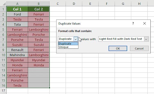
To highlight duplicate values between two columns using conditional formatting:

Select both columns of data.
Go to the Home tab and click on Conditional Formatting.
Choose Highlight Cells Rules and select Duplicate Values.
In the Duplicate Values dialog box, ensure Duplicate is selected.
Choose a formatting style (e.g., fill color) and click OK.

This will highlight all cells containing values that appear in both columns.

2.2. Highlighting Unique Values

To highlight unique values in one column compared to another using conditional formatting:

Select the column you want to analyze for unique values.
Go to the Home tab and click on Conditional Formatting.
Choose New Rule.
Select Use a formula to determine which cells to format.
Enter the formula =COUNTIF($B:$B,A1)=0, where A1 is the first cell in the selected column and $B:$B is the column to compare against.
Click Format to choose a formatting style (e.g., fill color) and click OK.

This will highlight all cells in the selected column that do not have a matching value in the comparison column.

2.3. Customizing Conditional Formatting Rules

You can customize conditional formatting rules to suit specific comparison needs:

Multiple Criteria: Combine multiple criteria to highlight cells based on more complex conditions.
Formula-Based Rules: Use custom formulas to define formatting rules that go beyond simple duplicate or unique value checks.
Color Scales: Apply color scales to visually represent the range of values in a column.

3. Using the Equals Operator for Column Comparison

The equals operator (=) in Excel allows you to perform cell-by-cell comparisons, returning TRUE if the values match and FALSE if they differ. This method provides a straightforward way to identify discrepancies between two columns.

3.1. Basic Cell Comparison

To compare two cells using the equals operator:

In a new column, enter the formula =A1=B1, where A1 and B1 are the first cells in the columns you want to compare.
Press Enter to display the result (TRUE or FALSE).
Drag the fill handle (the small square at the bottom-right of the cell) down to apply the formula to the remaining rows.

This will display TRUE for each row where the values in the corresponding cells match and FALSE where they differ.

3.2. Customizing Results with the IF Formula

To display custom messages instead of TRUE and FALSE, you can use the IF formula in conjunction with the equals operator:

In a new column, enter the formula =IF(A1=B1, "Match", "Mismatch"), where A1 and B1 are the first cells in the columns you want to compare.
Press Enter to display the result (Match or Mismatch).
Drag the fill handle down to apply the formula to the remaining rows.

This will display "Match" for each row where the values match and "Mismatch" where they differ.

3.3. Handling Different Data Types

When comparing columns with different data types (e.g., numbers and text), Excel may produce unexpected results. To ensure accurate comparisons, you may need to convert data types using functions like VALUE (to convert text to numbers) or TEXT (to format numbers as text).

4. Using the VLOOKUP Function for Column Comparison

The VLOOKUP function in Excel allows you to search for a value in one column and retrieve corresponding data from another column. This is particularly useful for comparing two columns and identifying matches or missing values.

4.1. Basic VLOOKUP Syntax

The syntax for the VLOOKUP function is:

=VLOOKUP(lookup_value, table_array, col_index_num, [range_lookup])

lookup_value: The value you want to search for.
table_array: The range of cells where you want to search.
col_index_num: The column number in the table_array from which to retrieve the result.
[range_lookup]: Optional. TRUE for approximate match (default), FALSE for exact match.

4.2. Comparing Columns with VLOOKUP

To compare two columns using VLOOKUP:

In a new column, enter the formula =VLOOKUP(A1, $B$1:$B$10, 1, FALSE), where A1 is the first cell in the column you want to search, $B$1:$B$10 is the range of cells in the comparison column, and 1 is the column index number (since we’re looking for the value itself).
Press Enter to display the result. If a match is found, the value from the comparison column will be displayed; otherwise, an error (#N/A) will be displayed.
Drag the fill handle down to apply the formula to the remaining rows.

4.3. Handling Errors with IFERROR

To handle errors (e.g., #N/A) when a match is not found, you can use the IFERROR function:

Modify the formula to =IFERROR(VLOOKUP(A1, $B$1:$B$10, 1, FALSE), "Not Found").
Press Enter to display the result. If a match is found, the value from the comparison column will be displayed; otherwise, "Not Found" will be displayed.
Drag the fill handle down to apply the formula to the remaining rows.

4.4. Using Wildcards for Partial Matches

In some cases, you may need to compare columns based on partial matches. You can use wildcards (* for any number of characters, ? for a single character) in conjunction with VLOOKUP to achieve this.

For example, to find values in column A that contain a specific substring found in column B:

Modify the formula to =IFERROR(VLOOKUP("*"&A1&"*", $B$1:$B$10, 1, FALSE), "Not Found").
Press Enter to display the result. If a partial match is found, the value from the comparison column will be displayed; otherwise, "Not Found" will be displayed.
Drag the fill handle down to apply the formula to the remaining rows.

5. Using the IF Formula for Column Comparison

The IF formula in Excel allows you to perform conditional tests and return different results based on whether the test is TRUE or FALSE. This is useful for creating custom comparison logic and displaying meaningful messages.

5.1. Basic IF Formula Syntax

The syntax for the IF formula is:

=IF(logical_test, value_if_true, value_if_false)

logical_test: The condition you want to test.
value_if_true: The value to return if the condition is TRUE.
value_if_false: The value to return if the condition is FALSE.

5.2. Comparing Columns with the IF Formula

To compare two columns using the IF formula:

In a new column, enter the formula =IF(A1=B1, "Same", "Different"), where A1 and B1 are the first cells in the columns you want to compare.
Press Enter to display the result ("Same" or "Different").
Drag the fill handle down to apply the formula to the remaining rows.

This will display "Same" for each row where the values match and "Different" where they differ.

5.3. Nested IF Statements for Multiple Conditions

You can use nested IF statements to create more complex comparison logic with multiple conditions:

In a new column, enter the formula =IF(A1=B1, "Same", IF(A1>B1, "A is greater", "B is greater")).
Press Enter to display the result.
Drag the fill handle down to apply the formula to the remaining rows.

This formula first checks if the values are the same. If not, it checks if the value in column A is greater than the value in column B, and displays the appropriate message.

6. Using the EXACT Formula for Column Comparison

The EXACT formula in Excel compares two strings and returns TRUE if they are exactly the same, including case, and FALSE otherwise. This is useful for case-sensitive comparisons.

6.1. Basic EXACT Formula Syntax

The syntax for the EXACT formula is:

=EXACT(text1, text2)

text1: The first string to compare.
text2: The second string to compare.

6.2. Comparing Columns with the EXACT Formula

To compare two columns using the EXACT formula:

In a new column, enter the formula =EXACT(A1, B1), where A1 and B1 are the first cells in the columns you want to compare.
Press Enter to display the result (TRUE or FALSE).
Drag the fill handle down to apply the formula to the remaining rows.

This will display TRUE for each row where the values are exactly the same (including case) and FALSE where they differ.

6.3. Case-Sensitive Comparisons

Unlike the equals operator (=), the EXACT formula is case-sensitive, making it suitable for scenarios where case matters.

For example, if cell A1 contains "Honda" and cell B1 contains "honda", the formula =EXACT(A1, B1) will return FALSE, while the formula =A1=B1 might return TRUE (depending on Excel’s settings).

7. Scenarios for Different Comparison Methods

Choosing the right column comparison method depends on your specific needs and the nature of your data. Here are some scenarios and recommended methods:

7.1. Comparing Two Columns Row-by-Row

Method: Equals Operator (=), IF Formula
Formulas:
- =IF(A2=B2, "Match", "Mismatch")
- =IF(A2<>B2, "No Match", "Match")
Use Case: Identifying differences between corresponding rows in two datasets.

7.2. Case-Sensitive Row-by-Row Comparison

Method: EXACT Formula
Formulas:
- =IF(EXACT(A2, B2), "Match", "Mismatch")
- =IF(EXACT(A2, B2), "Match", "No Match")
Use Case: Ensuring exact matches, including case, between two columns.

7.3. Comparing Multiple Columns for Row Matches

Method: AND, COUNTIF
Formulas:
- =IF(AND(A2=B2, A2=C2), "Complete Match", " ")
- =IF(COUNTIF($A2:$E2, $A2)=4, "Complete Match", " ") (where 4 is the number of columns being compared)
Use Case: Verifying that multiple columns have identical values in the same row.

7.4. Comparing Two Columns for Matches and Differences

Method: COUNTIF, MATCH, IFERROR
Formulas:
- =IF(COUNTIF($B:$B, $A2)=0, "Not Present in B", "Present in B")
- =IF(ISERROR(MATCH($A2, $B$2:$B$10, 0)), "Not Present in B", "Present in B")
Use Case: Finding unique values in one column compared to another.

7.5. Comparing Two Lists and Pulling Matching Data

Method: VLOOKUP, INDEX MATCH, XLOOKUP
Formulas:
- =VLOOKUP(D2, $A$2:$B$6, 2, FALSE)
- =INDEX($B$2:$B$6, MATCH($D2, $A$2:$A$6, 0))
- =XLOOKUP(D2, $A$2:$A$6, $B$2:$B$6)
Use Case: Extracting data from one list based on matches in another list.

7.6. Highlighting Row Matches and Differences

Method: Conditional Formatting, AND, COUNTIF
Formulas:
- =AND($A2=$B2, $A2=$C2)
- =COUNTIF($A2:$C2, $A2)=3 (where 3 is the number of columns being compared)
Use Case: Visually identifying rows with identical values across multiple columns.

8. Frequently Asked Questions (FAQs)

8.1. How do I compare two columns in Excel to see if they match?

You can use the equals operator (=) or the IF formula. For example, =IF(A1=B1, "Match", "Mismatch") will display “Match” if the values in cells A1 and B1 are the same and “Mismatch” if they are different.

8.2. Can I compare two columns in Excel using the Index-Match function?

Yes, you can use the INDEX and MATCH functions to compare two columns. This is particularly useful when you want to retrieve data from one column based on matches in another column. The formula would look something like this: =INDEX(ColumnB, MATCH(A1, ColumnA, 0)).

8.3. How do I compare multiple columns in Excel for duplicate values?

You can use conditional formatting to highlight duplicate values across multiple columns. Select all the columns, go to Home > Conditional Formatting > Highlight Cells Rules > Duplicate Values.

8.4. How do I compare two lists in Excel and find the matches?

You can use the VLOOKUP function or the COUNTIF function to compare two lists and find matches. For example, =COUNTIF(List2, A1) will count how many times the value in cell A1 appears in List2. If the result is greater than 0, it means there is a match.

8.5. How do I compare two columns in Excel and highlight the duplicates?

Select the two columns you want to compare. Go to Home > Conditional Formatting > Highlight Cells Rules > Duplicate Values. Choose a formatting style and click OK. Excel will highlight the duplicate values in both columns.

9. Conclusion: Choosing the Right Method for Your Needs

Comparing columns in Excel is a fundamental skill for data analysis, allowing you to validate data, identify trends, and make informed decisions. By mastering the techniques discussed in this guide, including conditional formatting, the equals operator, VLOOKUP, IF, and EXACT formulas, you can streamline your data analysis workflow and extract meaningful insights from your data.

At COMPARE.EDU.VN, we understand the importance of efficient and accurate data comparison. Whether you are a student, professional, or business owner, our resources are designed to help you make the most of Excel’s powerful comparison tools.

10. Call to Action: Explore More at COMPARE.EDU.VN

Ready to take your data analysis skills to the next level? Visit COMPARE.EDU.VN today to explore more in-depth guides, tutorials, and resources. Our comprehensive platform provides the tools and knowledge you need to make informed decisions and drive success in your academic, professional, and personal endeavors.

Address: 333 Comparison Plaza, Choice City, CA 90210, United States
WhatsApp: +1 (626) 555-9090
Website: COMPARE.EDU.VN

Discover the power of informed decision-making with compare.edu.vn.