Comparing two spreadsheets to reconcile data can be daunting. But with VLOOKUP, it becomes an efficient process. This article on COMPARE.EDU.VN offers a detailed, step-by-step guide on how to use VLOOKUP and other Excel functions to compare two spreadsheets, identify differences, and reconcile data effectively. Discover how to reconcile data, match values, and highlight discrepancies effortlessly.
1. What is VLOOKUP and Why Use It for Spreadsheet Comparison?
VLOOKUP (Vertical Lookup) is a powerful function in Excel that allows you to find a specific value in a column and return a corresponding value from another column in the same row. This is particularly useful when you need to compare two spreadsheets that share a common identifier, such as a customer ID or product code.
1.1. Benefits of Using VLOOKUP for Spreadsheet Comparison
- Efficiency: VLOOKUP automates the process of manually searching for matching values, saving you time and effort.
- Accuracy: By using VLOOKUP, you reduce the risk of human error that can occur when manually comparing large datasets.
- Scalability: VLOOKUP can handle large spreadsheets with thousands of rows, making it a suitable solution for businesses of all sizes.
- Flexibility: VLOOKUP can be used to compare various types of data, including text, numbers, and dates.
1.2. Use Cases for VLOOKUP in Data Comparison
- Reconciling financial data: Compare transaction records from two different systems to identify discrepancies.
- Matching customer information: Verify customer details across multiple databases to ensure data consistency.
- Comparing inventory lists: Identify differences in stock levels between two inventory reports.
- Validating product pricing: Compare product prices across different sales channels.
- Verifying order details: Ensure that order information is consistent between the sales and fulfillment departments.
2. Understanding the Basics of VLOOKUP
Before diving into the step-by-step guide, let’s understand the syntax and arguments of the VLOOKUP function.
2.1. VLOOKUP Syntax
The syntax for the VLOOKUP function is as follows:
=VLOOKUP(lookup_value, table_array, col_index_num, [range_lookup])2.2. VLOOKUP Arguments Explained
- lookup_value: The value you want to search for in the first column of the table_array.
- table_array: The range of cells that contains the data you want to search.
- col_index_num: The column number in the table_array from which you want to return a value.
- range_lookup: An optional argument that specifies whether you want to find an exact match or an approximate match. Use
FALSEfor an exact match andTRUEfor an approximate match. If omitted, it defaults toTRUE.
2.3. VLOOKUP vs. XLOOKUP
While VLOOKUP is a classic Excel function, XLOOKUP is a more modern and versatile alternative available in Excel 365 and later versions.
2.4. Key Differences Between VLOOKUP and XLOOKUP
- Flexibility: XLOOKUP can search both vertically and horizontally, while VLOOKUP is limited to vertical searches.
- Column Index: XLOOKUP doesn’t require specifying a column index number. Instead, you specify the return array directly.
- Error Handling: XLOOKUP has built-in error handling, allowing you to specify a value to return if no match is found.
- Performance: XLOOKUP is generally faster and more efficient than VLOOKUP, especially when dealing with large datasets.
- Syntax: XLOOKUP syntax is more intuitive and easier to understand than VLOOKUP syntax.
3. Step-by-Step Guide: How to Use VLOOKUP to Compare Two Spreadsheets
Here’s a detailed guide on how to use VLOOKUP to compare two spreadsheets.
3.1. Step 1: Set Up Your Data
First, organize your data in two separate Excel sheets within the same workbook. Ensure that both sheets have a common identifier column, such as “Customer ID” or “Product Code.” This common identifier will be used as the lookup_value in the VLOOKUP function.
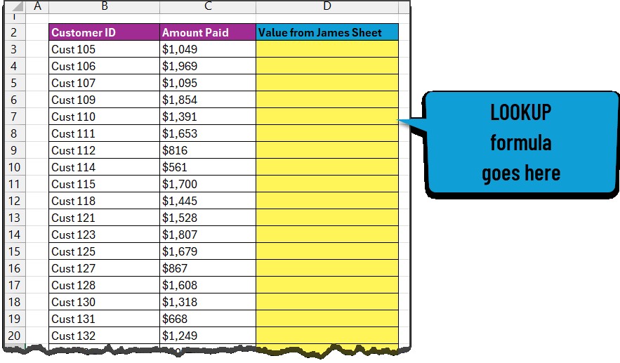
3.2. Step 2: Open the First Sheet and Insert the VLOOKUP Formula
In the first sheet, insert a new column where you want to display the matching values from the second sheet. In the first cell of this new column, enter the VLOOKUP formula.
For example, if you want to compare the “Amount Paid” column in both sheets based on “Customer ID,” the VLOOKUP formula in the first sheet would look like this:
=VLOOKUP(A2,'Sheet2'!$A:$B,2,FALSE)In this formula:
A2is the cell containing the first “Customer ID” in the first sheet.'Sheet2'!$A:$Bis the range of cells in the second sheet that contains the “Customer ID” and “Amount Paid” columns. The dollar signs ($) make the reference absolute, so it doesn’t change when you drag the formula down.2is the column number in the second sheet that contains the “Amount Paid” values (the second column in the range).FALSEensures that VLOOKUP looks for an exact match of the “Customer ID.”
3.3. Step 3: Apply the VLOOKUP Formula to All Rows
Drag the fill handle (the small square at the bottom-right corner of the cell) down to apply the VLOOKUP formula to all rows in the first sheet. This will populate the new column with the matching “Amount Paid” values from the second sheet.
3.4. Step 4: Handle #N/A Errors
If VLOOKUP cannot find a matching “Customer ID” in the second sheet, it will return a #N/A error. This indicates that the customer ID is missing in the second worksheet. You can use the IFERROR function to replace these errors with a more descriptive message, such as “ID Missing.”
Modify the VLOOKUP formula as follows:
=IFERROR(VLOOKUP(A2,'Sheet2'!$A:$B,2,FALSE),"ID Missing")3.5. Step 5: Compare the Values Using the IF Function
Now that you have the matching values from the second sheet in the first sheet, you can compare the values using the IF function. Insert another new column in the first sheet and enter the following formula in the first cell:
=IF(B2=C2,"Matching","Not Matching")In this formula:
B2is the cell containing the “Amount Paid” value in the first sheet.C2is the cell containing the matching “Amount Paid” value from the second sheet (obtained using VLOOKUP)."Matching"is the value that will be displayed if the two amounts are the same."Not Matching"is the value that will be displayed if the two amounts are different.
3.6. Step 6: Apply the IF Formula to All Rows
Drag the fill handle down to apply the IF formula to all rows in the first sheet. This will flag each row as either “Matching” or “Not Matching,” depending on whether the amounts in the two sheets are the same.
3.7. Step 7: Use Conditional Formatting to Highlight Discrepancies
To easily identify the “Not Matching” rows, you can use conditional formatting to highlight them.
- Select the entire range of data in the first sheet.
- Go to the “Home” tab on the Excel ribbon and click “Conditional Formatting.”
- Select “New Rule.”
- Choose “Use a formula to determine which cells to format.”
- Enter the following formula:
=$D2="Not Matching"(assuming the “Matching/Not Matching” column is column D). - Click “Format” and choose a background color to highlight the “Not Matching” rows.
- Click “OK” to apply the conditional formatting rule.
3.8. Step 8: Filter the Data to View Discrepancies
You can use Excel’s filtering feature to quickly view only the “Not Matching” rows.
- Select the header row in the first sheet.
- Go to the “Data” tab on the Excel ribbon and click “Filter.”
- Click the filter icon in the “Matching/Not Matching” column.
- Uncheck “Matching” to display only the “Not Matching” rows.
4. Alternative Techniques for Comparing Spreadsheets
While VLOOKUP is a powerful tool, there are other techniques you can use to compare spreadsheets.
4.1. Using the MATCH Function
The MATCH function can be used to find the position of a value in a range of cells. You can use MATCH in conjunction with IF to compare two spreadsheets.
=IF(ISNUMBER(MATCH(A2,'Sheet2'!$A:$A,0)),"Matching","Not Matching")This formula checks if the value in cell A2 of the first sheet exists in column A of the second sheet. If it does, the formula returns “Matching”; otherwise, it returns “Not Matching.”
4.2. Using Conditional Formatting with a Formula
You can use conditional formatting with a formula to highlight cells that are different between two spreadsheets.
- Select the range of cells you want to compare in the first sheet.
- Go to the “Home” tab on the Excel ribbon and click “Conditional Formatting.”
- Select “New Rule.”
- Choose “Use a formula to determine which cells to format.”
- Enter the following formula:
=A2<>'Sheet2'!A2(assuming you are comparing cell A2 in the first sheet with cell A2 in the second sheet). - Click “Format” and choose a background color to highlight the different cells.
- Click “OK” to apply the conditional formatting rule.
4.3. Using Excel’s “Compare Side by Side” Feature
Excel has a built-in “Compare Side by Side” feature that allows you to view two spreadsheets simultaneously and scroll through them in sync.
- Open both spreadsheets you want to compare.
- Go to the “View” tab on the Excel ribbon and click “View Side by Side.”
- If you want to scroll both spreadsheets simultaneously, click “Synchronous Scrolling.”
4.4. Using the Power Query Editor
Power Query Editor is a powerful data transformation and analysis tool in Excel. You can use it to compare two spreadsheets by merging them based on a common identifier and then identifying the differences.
- Open a new Excel workbook.
- Go to the “Data” tab on the Excel ribbon and click “Get Data” > “From File” > “From Workbook.”
- Select the first spreadsheet you want to compare and click “Import.”
- In the Power Query Editor, select the table containing the data and click “Close & Load To” > “Only Create Connection.”
- Repeat steps 2-4 for the second spreadsheet.
- Go to the “Data” tab and click “Get Data” > “Combine Queries” > “Merge.”
- Select the first table and the common identifier column.
- Select the second table and the corresponding common identifier column.
- Choose the “Full Outer” join type to include all rows from both tables.
- Click “OK.”
- Expand the second table to include the columns you want to compare.
- Add a custom column to compare the values in the two tables using the
IFfunction. - Close and load the merged table to a new sheet in the Excel workbook.
5. Best Practices for Spreadsheet Comparison
Here are some best practices to keep in mind when comparing spreadsheets.
5.1. Ensure Data Consistency
Before comparing spreadsheets, make sure that the data is consistent and accurate. Check for any errors, inconsistencies, or missing values that could affect the comparison results.
5.2. Use a Unique Identifier
Always use a unique identifier column, such as “Customer ID” or “Product Code,” to match the rows in the two spreadsheets. This ensures that you are comparing the correct records.
5.3. Clean Your Data
Clean your data by removing any unnecessary spaces, special characters, or formatting that could interfere with the comparison process.
5.4. Sort Your Data
Sort your data by the common identifier column to make it easier to identify any discrepancies.
5.5. Use Absolute References
When using formulas like VLOOKUP, use absolute references (e.g., $A$2) to prevent the references from changing when you copy the formula to other cells.
5.6. Test Your Formulas
Before applying your formulas to the entire dataset, test them on a small sample of data to ensure that they are working correctly.
5.7. Document Your Process
Document your spreadsheet comparison process, including the steps you took, the formulas you used, and any assumptions you made. This will make it easier to repeat the process in the future and to troubleshoot any issues that may arise.
6. Common Errors and Troubleshooting Tips
When comparing spreadsheets, you may encounter some common errors. Here are some troubleshooting tips to help you resolve them.
6.1. #N/A Error in VLOOKUP
The #N/A error in VLOOKUP indicates that the lookup value was not found in the table array. This can be caused by several factors, such as:
- The lookup value does not exist in the table array.
- The lookup value is misspelled or contains extra spaces.
- The table array is not correctly specified.
- The
range_lookupargument is set toFALSE(exact match) and the lookup value is not an exact match.
To resolve the #N/A error, check the following:
- Verify that the lookup value exists in the table array.
- Check for any spelling errors or extra spaces in the lookup value.
- Ensure that the table array is correctly specified and includes the lookup column.
- If you are using
FALSEfor exact match, make sure that the lookup value is an exact match. - Use the
IFERRORfunction to handle the#N/Aerror and display a more descriptive message.
6.2. Incorrect Results
If you are getting incorrect results when comparing spreadsheets, check the following:
- Verify that the formulas are correctly entered and that the references are accurate.
- Ensure that the data is consistent and accurate.
- Check for any formatting issues that could be affecting the comparison process.
- Test the formulas on a small sample of data to ensure that they are working correctly.
6.3. Performance Issues
If you are working with large spreadsheets, you may experience performance issues when comparing them. Here are some tips to improve performance:
- Use the
INDEXandMATCHfunctions instead of VLOOKUP, as they are generally faster. - Avoid using volatile functions, such as
NOW()andTODAY(), as they recalculate every time the spreadsheet is updated. - Disable automatic calculation and manually calculate the spreadsheet when needed.
- Use Excel’s “Evaluate Formula” feature to step through the formulas and identify any bottlenecks.
- Consider using Power Query Editor to perform the comparison, as it is designed to handle large datasets efficiently.
7. Real-World Examples of VLOOKUP in Action
To illustrate the practical applications of VLOOKUP, let’s explore a few real-world examples.
7.1. Example 1: Comparing Sales Data from Two Regions
A national retail company wants to compare sales data from its East and West Coast regions to identify top-performing products and areas for improvement.
- Sheet 1 (East Coast Sales): Contains columns for “Product ID,” “Product Name,” and “Sales Revenue.”
- Sheet 2 (West Coast Sales): Contains the same columns as Sheet 1.
By using VLOOKUP with “Product ID” as the lookup value, the company can quickly compare the sales revenue for each product in both regions, identify discrepancies, and make data-driven decisions about inventory management and marketing strategies.
7.2. Example 2: Reconciling Bank Statements with Accounting Records
A small business owner needs to reconcile their bank statements with their accounting records to ensure accuracy and detect any unauthorized transactions.
- Sheet 1 (Bank Statement): Contains columns for “Transaction Date,” “Transaction Description,” and “Transaction Amount.”
- Sheet 2 (Accounting Records): Contains the same columns as Sheet 1.
By using VLOOKUP with a combination of “Transaction Date” and “Transaction Amount” as the lookup value, the business owner can quickly identify matching transactions in both records, flag any discrepancies, and investigate potential errors or fraud.
7.3. Example 3: Validating Employee Data Across HR Systems
A large corporation is migrating its employee data from an old HR system to a new one. To ensure data integrity, they need to validate that all employee information has been transferred correctly.
- Sheet 1 (Old HR System): Contains columns for “Employee ID,” “Employee Name,” “Job Title,” and “Department.”
- Sheet 2 (New HR System): Contains the same columns as Sheet 1.
By using VLOOKUP with “Employee ID” as the lookup value, the corporation can quickly compare the employee information in both systems, identify any missing or incorrect data, and take corrective action to ensure a smooth and accurate migration.
8. Optimizing VLOOKUP for Large Datasets
When working with large datasets, VLOOKUP can become slow and inefficient. Here are some techniques to optimize VLOOKUP for better performance.
8.1. Use INDEX and MATCH Instead of VLOOKUP
The INDEX and MATCH functions can often be faster than VLOOKUP, especially when dealing with large datasets. INDEX returns the value of a cell in a table based on its row and column numbers, while MATCH finds the position of a value in a range of cells.
Here’s how to use INDEX and MATCH to achieve the same result as VLOOKUP:
=INDEX('Sheet2'!$B:$B,MATCH(A2,'Sheet2'!$A:$A,0))In this formula:
'Sheet2'!$B:$Bis the column containing the values you want to return.A2is the lookup value.'Sheet2'!$A:$Ais the column containing the lookup values.0specifies that you want an exact match.
8.2. Sort the Lookup Column
Sorting the lookup column in ascending order can significantly improve VLOOKUP’s performance, especially when using the approximate match option (i.e., when the range_lookup argument is set to TRUE or omitted).
8.3. Use Helper Columns
Creating helper columns can sometimes simplify complex VLOOKUP formulas and improve performance. For example, you can create a helper column that concatenates multiple columns into a single lookup value.
8.4. Avoid Volatile Functions
Volatile functions, such as NOW() and TODAY(), recalculate every time the spreadsheet is updated, which can slow down VLOOKUP’s performance. Avoid using volatile functions in your VLOOKUP formulas whenever possible.
8.5. Use Excel Tables
Using Excel tables can improve VLOOKUP’s performance by automatically adjusting the table range when you add or remove rows. To create an Excel table, select your data range and press Ctrl+T.
9. VLOOKUP Alternatives in Other Spreadsheet Software
While VLOOKUP is a staple in Excel, other spreadsheet software offers similar functions with slightly different names and syntax.
9.1. Google Sheets: VLOOKUP
Google Sheets has a VLOOKUP function that is virtually identical to Excel’s VLOOKUP. The syntax and arguments are the same, so you can use the same formulas in both programs.
9.2. LibreOffice Calc: VLOOKUP
LibreOffice Calc also has a VLOOKUP function that works similarly to Excel’s VLOOKUP. The syntax and arguments are the same, but there may be some minor differences in how the function handles errors and edge cases.
9.3. Apache OpenOffice Calc: VLOOKUP
Apache OpenOffice Calc has a VLOOKUP function that is similar to Excel’s VLOOKUP, but there may be some differences in the syntax and arguments. Refer to the Apache OpenOffice Calc documentation for more information.
10. Advanced VLOOKUP Techniques
Once you’ve mastered the basics of VLOOKUP, you can explore some advanced techniques to take your spreadsheet comparison skills to the next level.
10.1. Using VLOOKUP with Multiple Criteria
You can use VLOOKUP with multiple criteria by creating a helper column that concatenates the criteria into a single lookup value.
For example, if you want to compare data based on both “Customer ID” and “Product ID,” you can create a helper column in both spreadsheets that concatenates these two columns:
=A2&B2Then, use this helper column as the lookup value in your VLOOKUP formula.
10.2. Using VLOOKUP with Wildcards
You can use wildcards in your VLOOKUP formulas to find partial matches. The two wildcards available in Excel are:
*: Matches any sequence of characters.?: Matches any single character.
For example, if you want to find all product names that start with “A,” you can use the following VLOOKUP formula:
=VLOOKUP("A*",'Sheet2'!$A:$B,2,FALSE)10.3. Using VLOOKUP to Return Multiple Values
You can use VLOOKUP to return multiple values by combining it with the COLUMN function. The COLUMN function returns the column number of a cell.
For example, if you want to return the “Product Name” and “Product Price” from the second sheet based on “Product ID,” you can use the following formulas:
=VLOOKUP(A2,'Sheet2'!$A:$C,2,FALSE) 'Returns Product Name
=VLOOKUP(A2,'Sheet2'!$A:$C,3,FALSE) 'Returns Product Price
You can also use the COLUMN function to make the formulas more dynamic:
=VLOOKUP(A2,'Sheet2'!$A:$C,COLUMN(B1),FALSE) 'Returns Product Name
=VLOOKUP(A2,'Sheet2'!$A:$C,COLUMN(C1),FALSE) 'Returns Product Price
10.4. Using VLOOKUP with Named Ranges
Using named ranges can make your VLOOKUP formulas more readable and easier to maintain. To create a named range, select the range of cells you want to name and then type the name in the name box (located to the left of the formula bar).
Then, you can use the named range in your VLOOKUP formula:
=VLOOKUP(A2,ProductData,2,FALSE)In this formula, “ProductData” is the named range that refers to the table array.
11. Why COMPARE.EDU.VN is Your Ultimate Comparison Resource
At COMPARE.EDU.VN, we understand the challenges of making informed decisions when faced with multiple options. Our mission is to provide you with comprehensive and objective comparisons across a wide range of products, services, and ideas, empowering you to make confident choices.
11.1. Comprehensive and Objective Comparisons
Our team of experts meticulously researches and analyzes each option, providing you with detailed comparisons that highlight the key differences, advantages, and disadvantages. We strive to present the information in a clear and unbiased manner, allowing you to form your own informed opinions.
11.2. Wide Range of Categories
Whether you’re comparing universities, financial products, software solutions, or travel destinations, COMPARE.EDU.VN has you covered. We offer comparisons across a diverse range of categories, ensuring that you can find the information you need, no matter what your decision-making process entails.
11.3. User Reviews and Ratings
In addition to our expert comparisons, we also provide user reviews and ratings to give you a well-rounded perspective. Hear from real people who have experience with the products or services you’re considering, and get valuable insights that can help you make the right choice.
11.4. Easy-to-Use Interface
Our website is designed with you in mind. We offer an intuitive and user-friendly interface that makes it easy to find the comparisons you’re looking for and navigate through the information.
11.5. Constantly Updated Information
We understand that the world is constantly changing, and new products and services are emerging all the time. That’s why we’re committed to keeping our comparisons up-to-date, ensuring that you have the latest information at your fingertips.
12. FAQ: Frequently Asked Questions About VLOOKUP and Spreadsheet Comparison
12.1. Can VLOOKUP compare data in two different Excel files?
Yes, VLOOKUP can compare data in two different Excel files, but you need to ensure that both files are open when you run the formula. The syntax for referencing a different file is ='[Filename.xlsx]Sheetname'!Range.
12.2. How do I handle case-sensitive comparisons with VLOOKUP?
VLOOKUP is not case-sensitive by default. To perform a case-sensitive comparison, you can use the EXACT function within an array formula.
12.3. What is the difference between VLOOKUP and HLOOKUP?
VLOOKUP searches for a value in the first column of a table and returns a value from the same row. HLOOKUP searches for a value in the first row of a table and returns a value from the same column.
12.4. Can I use VLOOKUP to compare data in different sheets of the same Excel file?
Yes, you can use VLOOKUP to compare data in different sheets of the same Excel file. Simply reference the other sheet in the table_array argument.
12.5. How do I compare two columns in Excel and highlight the differences?
You can use conditional formatting with a formula to compare two columns in Excel and highlight the differences. Select the range of cells in one column, go to Conditional Formatting > New Rule > Use a formula to determine which cells to format, and enter a formula like =$A1<>$B1 (assuming the columns are A and B).
12.6. What is the best way to compare two Excel files for differences?
Besides VLOOKUP, you can use Excel’s “Compare Side by Side” feature, conditional formatting, or Power Query to compare two Excel files for differences.
12.7. How can I find matching values in two Excel sheets?
You can use VLOOKUP or the MATCH function to find matching values in two Excel sheets.
12.8. What are the limitations of VLOOKUP?
Limitations of VLOOKUP include: it only searches in the first column, it can be slow with large datasets, and it doesn’t handle errors gracefully without additional functions like IFERROR.
12.9. How do I troubleshoot #N/A errors in VLOOKUP?
Check that the lookup value exists in the table array, verify the spelling, ensure the table array is correct, and confirm that you’re using the correct match type (exact or approximate).
12.10. What is the alternative to VLOOKUP in Excel?
Alternatives to VLOOKUP in Excel include INDEX and MATCH, XLOOKUP (in Excel 365 and later), and Power Query.
Conclusion
Comparing two spreadsheets doesn’t have to be a headache. By mastering VLOOKUP and other comparison techniques, you can efficiently reconcile data, identify discrepancies, and make informed decisions. Remember to visit COMPARE.EDU.VN for more comprehensive comparisons and resources to help you make the best choices.
Ready to streamline your spreadsheet comparisons and make data-driven decisions? Visit COMPARE.EDU.VN today to explore our comprehensive comparison tools and resources. Our team of experts is dedicated to providing you with the information you need to make confident choices.
Contact Us:
Address: 333 Comparison Plaza, Choice City, CA 90210, United States
WhatsApp: +1 (626) 555-9090
Website: COMPARE.EDU.VN
Don’t let data discrepancies hold you back. Empower yourself with the knowledge and tools you need to succeed. Visit compare.edu.vn and start comparing today!